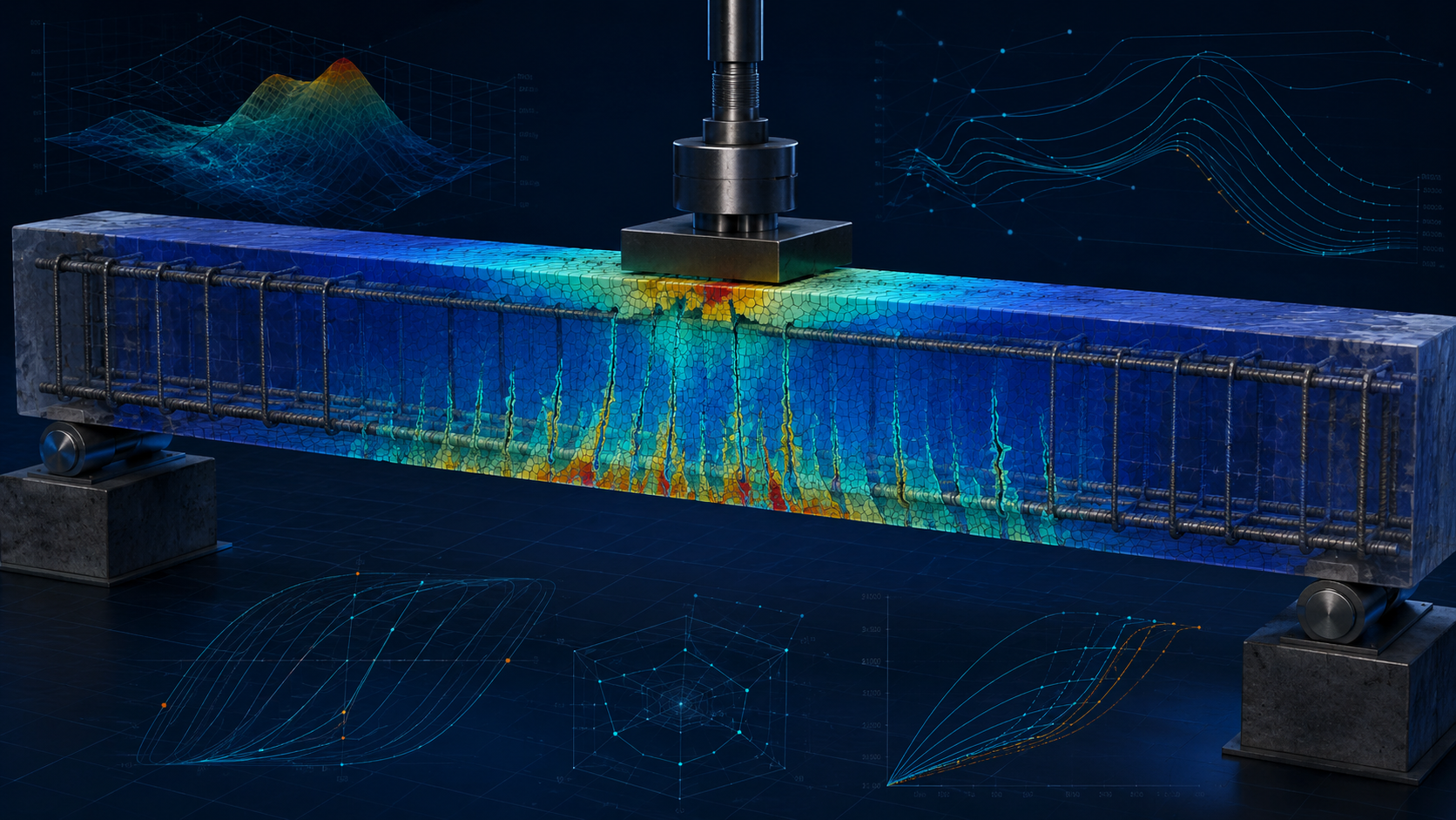
Concrete Damage Plasticity (CDP) is one of the most widely used concrete constitutive models in Abaqus, but it is also one of the easiest models to misuse. The difficulty is not finding five plasticity parameters on the internet. The real engineering problem is building a consistent material definition in which the plasticity parameters, compression hardening, tension stiffening, damage evolution, element size, solver settings, and validation response all describe the same concrete behaviour.
This guide is written for researchers, postgraduate students, and practising engineers who need to calibrate a CDP material model for a reinforced-concrete or plain-concrete finite element analysis. The objective is not to provide a universal parameter table. It is to show how the calibration workflow should be organised, checked, and defended.
How should Concrete Damage Plasticity parameters and uniaxial material data be defined, checked, and calibrated in Abaqus so that the numerical response remains physically interpretable and suitable for validation?
1. Why CDP calibration is harder than entering five parameters
Abaqus describes the concrete damaged plasticity model as a continuum, plasticity-based damage model for concrete and other quasi-brittle materials. The model combines plasticity with tensile and compressive stiffness degradation and is available in both Abaqus/Standard and Abaqus/Explicit. The plasticity definition alone is not a complete concrete model. Compression hardening and tension stiffening are required, while tensile and compressive damage definitions can be added to represent stiffness degradation.
This distinction matters because many failed CDP models begin with a five-value table copied from a paper. The analyst then assumes that the dilation angle, eccentricity, biaxial-to-uniaxial strength ratio, yield-surface shape factor, and viscosity parameter are the material model. They are not. These parameters control the plastic flow potential, yield surface, and viscoplastic regularisation. The uniaxial tensile and compressive response still has to be defined consistently.
Do not calibrate the five plasticity parameters in isolation. Treat CDP as one coupled material definition: elasticity + compression hardening + tension stiffening + optional damage + plasticity parameters + mesh and solver context.
2. Start from the response you need to reproduce
Before editing the material definition, decide what the model is expected to reproduce. Peak load, initial stiffness, post-peak softening, cyclic degradation, crack localisation, residual displacement, crushing zone, and energy dissipation are different calibration targets.
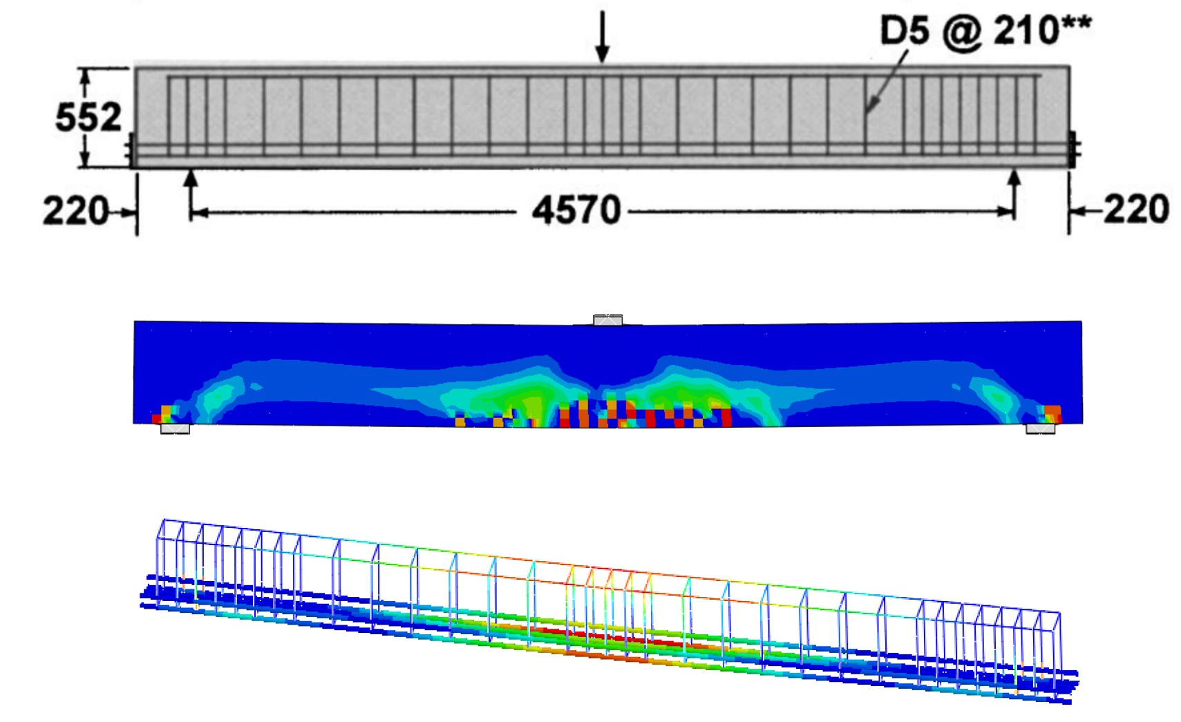
For a reinforced-concrete beam under concentrated loading, a practical validation set may include the load-displacement curve, first-cracking region, peak load, post-peak response, and the observed failure mode. For a wall or frame under cyclic loading, the hysteresis loop, pinching, stiffness degradation, accumulated damage, and residual drift may be more important. A parameter set that reproduces one response quantity is not automatically validated for another structural problem.
| Calibration target | Primary evidence | Typical sensitivity |
|---|---|---|
| Initial stiffness | Elastic slope / service response | Elastic modulus, boundary conditions, reinforcement stiffness |
| Peak load | Maximum measured resistance | Compression and tension data, confinement, interaction assumptions |
| Post-peak response | Softening branch | Tension stiffening, compression softening, damage, mesh |
| Crack or damage localisation | Observed failure pattern | Mesh, tensile law, damage variables, structural detailing |
| Cyclic degradation | Hysteresis and stiffness loss | Damage evolution, loading path, viscosity, interaction assumptions |
3. The five CDP plasticity parameters
The Concrete Damaged Plasticity definition contains parameters associated with the flow potential, yield surface, and viscosity. Abaqus accepts the dilation angle, flow-potential eccentricity, the ratio of initial equibiaxial compressive yield stress to initial uniaxial compressive yield stress, the ratio controlling the second stress invariant on the tensile and compressive meridians, and a viscosity parameter.
Dilation angle, ψ
The dilation angle controls the nonassociated plastic flow potential and strongly influences volumetric expansion and the apparent shear-related response of the concrete model. In structural simulations it can affect load capacity, confinement sensitivity, and post-yield deformation. A larger value should not be used simply because it improves agreement with peak load. If the parameter is being adjusted, record which response quantity changes and whether the resulting deformation mechanism remains credible.
Flow-potential eccentricity, ε
The eccentricity controls the rate at which the hyperbolic flow potential approaches its asymptote. Abaqus defines it as part of the Drucker-Prager hyperbolic flow potential. In many models this parameter is left at a commonly used value without sensitivity analysis. That may be acceptable when the adopted value is justified, but it should not be confused with a directly measured concrete property.
fb0/fc0
This ratio relates the initial equibiaxial compressive yield stress to the initial uniaxial compressive yield stress. It influences the multiaxial yield surface and therefore becomes important when the concrete experiences a non-uniaxial stress state. The parameter should be treated as part of the multiaxial strength description, not as a tuning coefficient for a single load-displacement curve.
Kc
The yield-surface shape parameter controls the ratio of the second stress invariant on the tensile meridian to that on the compressive meridian at initial yield. Its role becomes more important when the structural response includes complex multiaxial stress states. As with fb0/fc0, changing Kc to fix a poor global response may be hiding an error elsewhere in the model.
Viscosity parameter, μ
The viscosity parameter introduces viscoplastic regularisation. In Abaqus/Standard, a nonzero viscosity can help regularise the constitutive equations and improve convergence in softening problems. The numerical benefit is real, but the parameter can also alter the response if it is too large relative to the loading time scale. Therefore, viscosity should be checked through a sensitivity study rather than used as an invisible convergence switch.
4. Compression hardening: what Abaqus expects
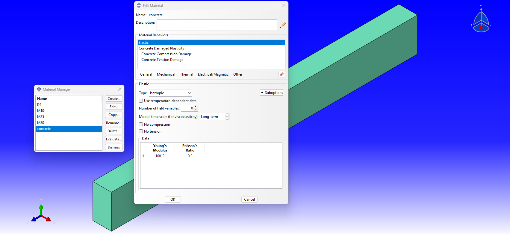
For Concrete Damaged Plasticity, Abaqus requires compression hardening data. The input is defined in terms of compressive yield stress and inelastic strain. This is one of the most important data-conversion steps in the entire calibration workflow.
If experimental data are available as total strain and stress, the analyst should not paste the total strain directly into the inelastic-strain column. The inelastic strain is obtained by removing the elastic strain contribution associated with the undamaged elastic modulus:
where εc,in is the compressive inelastic strain used in the hardening definition, εc,total is the measured or adopted total compressive strain, σc is the compressive stress, and E0 is the initial elastic modulus.
Check the sign convention and the exact Abaqus data convention used in the CAE interface or keyword definition. More importantly, inspect the converted table before running the model. Inelastic strain should be physically ordered and the hardening data should not contain accidental reversals caused by spreadsheet errors, inconsistent signs, duplicated points, or mixed units.
A practical compression-data check
- Plot the original stress-total strain curve.
- Calculate the elastic strain σ/E0 for each point.
- Calculate the inelastic strain.
- Plot stress against inelastic strain.
- Check monotonic ordering of the input variable.
- Confirm that the first plastic point is consistent with the adopted yield definition.
- Verify units before copying the data to Abaqus.
When a model shows excessive compressive capacity, delayed softening, or unexpected localisation, do not adjust the dilation angle first. Recheck the compression curve, confinement conditions, reinforcement interaction, and the conversion from total strain to inelastic strain.
5. Tension stiffening and cracking strain
Abaqus requires a tension-stiffening definition for the CDP model. The tensile response after cracking is a major source of mesh sensitivity and modelling uncertainty, especially when the model is used to predict crack localisation or post-peak response.
Depending on the selected definition, tensile softening can be introduced using stress versus cracking strain or through a displacement/fracture-energy-based regularisation. For a strain-based definition, the cracking strain is related to the total tensile strain after removal of the elastic contribution:
The tension-stiffening law should represent the intended physical idealisation. In reinforced concrete, post-cracking tensile behaviour may be influenced by bond and reinforcement interaction at the structural scale. In plain concrete or local fracture studies, a fracture-energy-based description may be more appropriate. The important point is to identify what the chosen softening law represents.
Why the tensile law is mesh sensitive
When post-peak softening is defined directly in terms of strain, the energy dissipated in a localised band can change with element size. A refined mesh can localise damage into a smaller physical width and produce a different structural response. Therefore, a CDP model that matches one experiment with one mesh cannot be declared mesh independent without a sensitivity study.
Never calibrate tension stiffening against one mesh and then change the element size substantially without repeating the structural validation.
6. Tensile and compressive damage variables
The CDP model can include tensile and compressive stiffness degradation through damage variables. Abaqus provides separate tension and compression damage definitions, and the corresponding field outputs include DAMAGET and DAMAGEC. The scalar stiffness degradation output SDEG is also available for the CDP model.
A damage variable is not the same thing as a visible physical crack width. A contour of DAMAGET should therefore not be labelled automatically as a crack pattern without explaining the constitutive meaning and validation basis. Damage contours are useful for comparing localisation zones and structural failure mechanisms, but they should be interpreted together with stress, strain, displacement, reinforcement response, and experimental evidence.
Damage input also affects unloading and stiffness degradation. If a model is used under cyclic loading, this becomes particularly important. A model may reproduce monotonic peak load while giving unrealistic hysteresis because the degradation behaviour and loading path have not been calibrated.
7. A practical CDP calibration workflow
The following sequence is more reliable than changing several parameters at the same time.
Step 1 — Verify the structural model before nonlinear calibration
Check geometry, section assignments, reinforcement, constraints, contact, embedded regions, supports, and load application. Run a simplified elastic or reduced-nonlinearity check when possible. A wrong boundary condition can easily be mistaken for a CDP problem.
Step 2 — Establish the elastic response
Confirm elastic modulus and Poisson's ratio and compare the initial numerical stiffness with the reference response. If the initial slope is wrong, changing damage or dilation will not fix the underlying problem.
Step 3 — Build and inspect the compression hardening data
Convert the adopted stress-strain data to the required Abaqus inelastic-strain form. Plot the table and check ordering, signs, units, and the location of the peak and softening branch.
Step 4 — Define the tensile law
Select a tension-stiffening or fracture-energy idealisation that matches the problem. Document whether the model is intended to represent a structural reinforced-concrete response or local concrete fracture behaviour.
Step 5 — Add damage only with a defined purpose
Define tensile and compressive damage when stiffness degradation is part of the response being reproduced. Check the relationship between the damage tables and the corresponding tensile and compressive constitutive curves.
Step 6 — Select the plasticity parameters
Adopt literature, experimental, or established modelling values as a starting point where justified. Then perform targeted sensitivity studies. Change one parameter family at a time and record the response quantity affected.
Step 7 — Check mesh sensitivity
Repeat the analysis with at least one refined or modified mesh in the critical response zone. Compare the engineering output that matters: peak load, residual displacement, damage localisation, dissipated energy, or another defined quantity.
Step 8 — Validate the structural response
Compare the numerical result with an independent reference. A useful validation includes both a global response curve and a local or qualitative failure measure where possible.
8. Mesh density is part of CDP calibration
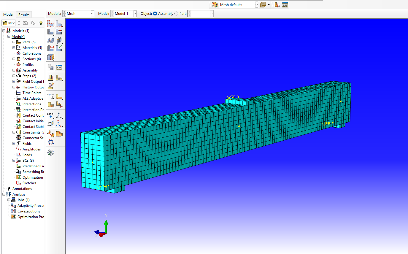
Concrete softening and damage localisation make mesh strategy part of the constitutive calibration problem. The same material table can produce different local damage patterns and post-peak response when the characteristic element size changes substantially.
Use a mesh strategy based on the response quantity. A global load-displacement study may converge before a local damage contour converges. Conversely, a very fine mesh may create a computationally expensive model without improving the engineering conclusion if the constitutive softening law is not appropriately regularised.
| Mesh level | Purpose | What to compare |
|---|---|---|
| Coarse | Initial screening and model debugging | Response trend, boundary-condition behaviour, gross deformation |
| Medium | Main engineering response assessment | Peak load, displacement, damage zone, solver behaviour |
| Fine / locally refined | Convergence confirmation | Change in the selected validation quantity and localisation pattern |
9. Solver choice and the viscosity parameter
CDP is available in Abaqus/Standard and Abaqus/Explicit. Solver choice should be based on the physics and numerical characteristics of the problem, not on the idea that one solver is universally better for concrete.
Abaqus/Standard may be appropriate for many static and quasi-static nonlinear analyses, but severe softening and localisation can make convergence difficult. The CDP viscosity parameter provides viscoplastic regularisation and can improve convergence, but the numerical response should be checked for sensitivity to the selected value.
Abaqus/Explicit avoids the global Newton equilibrium iterations used by the implicit procedure and can be useful for highly nonlinear contact, severe damage, and complex transient problems. When Explicit is used for a quasi-static concrete problem, the loading rate and energy balance must be checked so that inertial effects do not dominate the intended response.
If increasing μ is the only reason the model converges, compare multiple viscosity values and verify that the primary structural response remains stable. Numerical convergence and physical validation are separate requirements.
10. Output variables that help evaluate a CDP model
Do not judge the model only from a von Mises stress contour. Useful CDP-related output variables include:
| Output | Engineering use |
|---|---|
DAMAGET | Tensile damage variable; review localisation and stiffness degradation in tension. |
DAMAGEC | Compressive damage variable; review compression-related degradation zones. |
SDEG | Overall scalar stiffness degradation variable for the material model. |
PEEQ | Equivalent plastic strain in uniaxial compression for CDP output interpretation. |
| Stress and strain components | Check whether the local stress state is consistent with the assumed failure mechanism. |
| Displacement / reaction force | Build the global structural response used for validation. |
The output should be selected before the final analysis. If the validation requires a load-displacement curve, define the history output and reference points needed to construct the curve before running a large parametric study.
11. Validation: what should be compared?
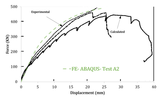
Parameter values are not validation evidence. The model should be judged against the response it was designed to reproduce.
Global validation
- Initial stiffness.
- Peak load or resistance.
- Displacement at peak load.
- Post-peak trend.
- Residual response where relevant.
- Hysteresis and energy dissipation for cyclic problems.
Local or mechanism-based validation
- Location of the critical damage or cracking region.
- Compression crushing zone.
- Reinforcement yielding region.
- Failure mode.
- Sequence of observed damage development where experimental evidence exists.
A useful model does not need perfect agreement at every point. It needs a transparent explanation of the remaining differences and evidence that the dominant structural mechanism has been captured.
12. Common CDP calibration errors
Copying the five parameters from an unrelated paper
Symptom: the model runs but the structural response is inconsistent. Check: whether the original study had comparable concrete strength, confinement, stress state, loading path, solver, and calibration target.
Entering total strain as inelastic strain
Symptom: compression hardening begins at the wrong strain level or the constitutive response becomes inconsistent. Check: the conversion from total strain to inelastic strain using the initial elastic modulus.
Using a universal tension-stiffening curve
Symptom: crack localisation or post-peak response changes strongly with mesh size. Check: what the tensile law represents and whether a fracture-energy or displacement-based regularisation is more appropriate.
Calling DAMAGET a crack width
Symptom: damage contours are presented as experimentally measured crack openings. Check: the constitutive meaning of the damage variable and compare the localisation pattern with independent evidence.
Increasing viscosity until the model converges
Symptom: the job converges only for a relatively large μ. Check: multiple viscosity values and compare the primary response curve, energy, and loading-time scale.
Calibrating material parameters before fixing supports and contact
Symptom: the CDP table is repeatedly changed to correct stiffness or peak load. Check first: boundary conditions, reinforcement interaction, contact, section assignments, and load application.
Validating only one contour image
Symptom: the colour contour looks plausible but there is no quantitative comparison. Check: load-displacement response, peak load, failure mechanism, and mesh sensitivity.
13. Related Numerical Archive models
Numerical Archive also includes reinforced-concrete slab, frame, joint, and other nonlinear concrete resources. These models can be useful when the research problem requires a structural configuration closer to the target study.
14. Engineering checklist before accepting a CDP model
- The validation quantity is defined before calibration.
- Elastic modulus and initial stiffness are checked.
- Compression data are converted to the Abaqus inelastic-strain definition correctly.
- Tension-stiffening data represent a documented physical idealisation.
- Damage tables are consistent with the tensile and compressive constitutive response.
- The dilation angle is not being used to hide a boundary-condition or material-data error.
- fb0/fc0 and Kc are treated as multiaxial yield-surface parameters.
- Viscosity sensitivity is checked when a nonzero μ is used.
- The mesh is justified for the selected response quantity.
- At least one mesh sensitivity comparison is performed in the critical region.
- DAMAGET and DAMAGEC are interpreted as constitutive damage variables, not direct crack-width measurements.
- The global structural response is compared with independent evidence.
- The failure mechanism or damage location is also reviewed where evidence is available.
- Calibration changes are documented one parameter family at a time.
15. Final recommendations
A credible Concrete Damage Plasticity model is not defined by a popular set of five parameters. It is defined by a traceable calibration process.
For a thesis, research paper, or engineering study, report the elastic properties, compression hardening data, tensile softening definition, damage assumptions, plasticity parameters, viscosity value, element type, characteristic mesh size, solver procedure, and the validation quantities used to accept the model.
The strongest CDP model is not the one that produces the most dramatic damage contour. It is the one for which the analyst can explain why the material data were defined that way, which response was calibrated, how mesh and solver effects were checked, and where the model remains uncertain.
References
- Dassault Systèmes SIMULIA — Concrete Damaged Plasticity.
- Dassault Systèmes SIMULIA — *CONCRETE DAMAGED PLASTICITY keyword reference.
- Dassault Systèmes SIMULIA — *CONCRETE COMPRESSION HARDENING.
- Dassault Systèmes SIMULIA — *CONCRETE TENSION STIFFENING.
- Dassault Systèmes SIMULIA — *CONCRETE TENSION DAMAGE.
- Dassault Systèmes SIMULIA — *CONCRETE COMPRESSION DAMAGE.
- Dassault Systèmes SIMULIA — CDP element integration-point output variables.