Abaqus errors are rarely random. Most job terminations are the solver’s way of reporting that the model has become inconsistent, unstable, excessively nonlinear, or numerically difficult to continue. The fastest way to fix an Abaqus error is not to change every solver setting until the job runs. It is to identify which part of the model is causing the failure and why.
This practical guide reviews common Abaqus errors and explains a diagnostic workflow for each one. The focus is on errors that frequently stop structural, mechanical, contact, damage, and nonlinear analyses: Missing Property Definition, Time increment required is less than the minimum specified, Too many attempts made for this increment, No density has been specified, numerical singularity, zero pivot, excessive distortion, and jobs that require an excessive number of increments.
Engineering note: An error message is usually the final symptom, not the root cause. Before changing time increments, convergence controls, stabilization, or solver type, inspect the model region, contact pair, material state, and load history active immediately before the failure.
How to Diagnose an Abaqus Error Before Changing the Model
A disciplined troubleshooting workflow saves more time than trial-and-error changes. When a job stops, begin with the files and diagnostics produced by Abaqus rather than immediately reopening the Step editor.
- Read the final job message. Record the exact error text and the step, increment, and time at which the analysis stopped.
- Open Job Diagnostics or the relevant message output. Review warnings, residual information, severe discontinuities, contact changes, and element-related messages.
- Identify the last successful increment. Compare the model immediately before failure with the failed state.
- Locate the active region. Determine where plasticity, damage, contact, large deformation, or high reaction forces are evolving.
- Check units and magnitudes. Verify force, displacement, density, modulus, yield stress, fracture energy, and geometric dimensions in one consistent unit system.
- Change one cause at a time. Do not simultaneously change mesh, material data, contact, step controls, and solver settings; otherwise, you will not know which change solved the problem.
For nonlinear Abaqus/Standard analyses, the solver repeatedly checks whether equilibrium and solution corrections satisfy the convergence criteria. If an increment is too difficult, automatic incrementation may cut back the time increment and retry. When repeated cutbacks still cannot produce a converged state, the analysis eventually terminates. The correct response is usually to diagnose the nonlinearity or modeling issue rather than simply forcing smaller increments indefinitely.
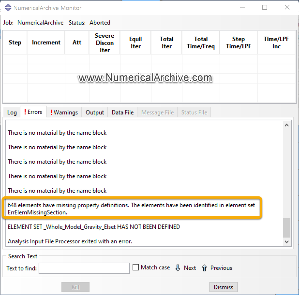
1. Missing Property Definition Error in Abaqus
The Missing Property Definition error usually means that one or more deformable regions do not have the section or property information required by the selected element formulation. In practical models, the cause is often an incomplete section assignment, an incorrect region selection, or a property assignment that was lost after geometry or partition changes.
Common Causes
- A solid, shell, beam, membrane, or truss region has no section assignment.
- A section was created but never assigned to the intended region.
- Partitioning or geometry edits changed the region and invalidated a previous assignment.
- The selected section type is incompatible with the element or part representation.
- A model contains orphaned or newly imported regions that were not included in the original property assignment.
Do not assume that creating a material is enough. Abaqus needs the complete chain from material definition to section definition and section assignment. For beam and truss models, also confirm that the selected element family and section definition are consistent with the intended structural representation.

How to Fix It
- Open the Property module.
- Review section assignments for the entire part or assembly region named in the warning.
- Display section assignments visually and look for unassigned faces, cells, edges, or wire regions.
- Confirm that the section references the correct material.
- After remeshing or geometry modification, verify that the assignment still covers the intended region.

Do not fix this error by changing the solver. Missing property information is a model-definition problem. The analysis procedure cannot compensate for a region that does not have the required section data.
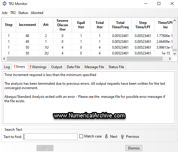
2. Time Increment Required Is Less Than the Minimum Specified
The “Time increment required is less than the minimum specified” message is one of the most common Abaqus/Standard convergence errors. It means that the solver has repeatedly reduced the increment while trying to find a converged equilibrium state, but the increment required to continue has become smaller than the minimum allowed in the step.
The minimum increment is not usually the root cause. The real question is: why does the current state require repeated cutbacks?
Common Causes
- Contact instability: initial overclosure, poor surface definition, contact chattering, abrupt opening and closing, or inappropriate contact stiffness.
- Excessive loading: a large force or displacement is applied too rapidly within the step.
- Material softening or damage: the tangent stiffness changes sharply as cracking, crushing, plastic localization, or damage evolves.
- Severe element distortion: large deformation produces poor element geometry or difficult element calculations.
- Unstable structural response: snap-through, buckling, local instability, or loss of stiffness may not be suitable for a conventional static procedure.
- Inconsistent units or unrealistic material data: an incorrect modulus, density, yield stress, fracture energy, or load magnitude can make the model numerically extreme.
- Boundary-condition problems: incompatible constraints, unintended rigid motion, or overconstraint may prevent equilibrium.
Why Reducing the Minimum Increment Is Not Always a Fix
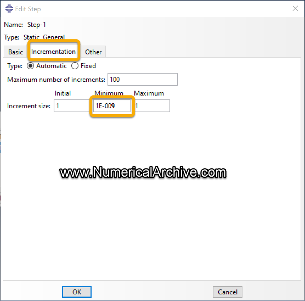
Changing the minimum increment from its default value to a very small value such as 1e-9 may allow Abaqus to attempt additional cutbacks. However, this can simply force the solver to spend more time trying to pass through the same unstable state. If contact, material behavior, mesh distortion, or structural instability is the real cause, a smaller minimum increment does not correct the model.
Practical Diagnostic Workflow
- Find the last converged increment and note the step time.
- Review contact status and severe discontinuities near the failure.
- Plot reaction force, displacement, stress, plastic strain, damage, and contact variables through the last successful increments.
- Inspect elements in the active nonlinear region for distortion or localization.
- Verify the unit system and the magnitude of all material and load data.
- Apply the load more smoothly or over a longer step if the physical problem permits it.
- Use automatic stabilization only when it is physically and numerically justified, and review the stabilization energy.
- Consider an alternative procedure if the model contains strong instability, complex evolving contact, or severe discontinuities.
If the problem is physically suitable for an explicit procedure, Abaqus/Explicit may be more robust for severe contact and highly nonlinear deformation. In that case, the analysis is controlled by the explicit stable time increment rather than Abaqus/Standard equilibrium iterations. When a small group of elements controls the explicit increment, carefully applied mass scaling in Abaqus may improve computational efficiency.
Do not confuse the Abaqus/Standard minimum-increment error with a small stable time increment in Abaqus/Explicit. They are different numerical issues and should be diagnosed differently.
3. Too Many Attempts Made for This Increment
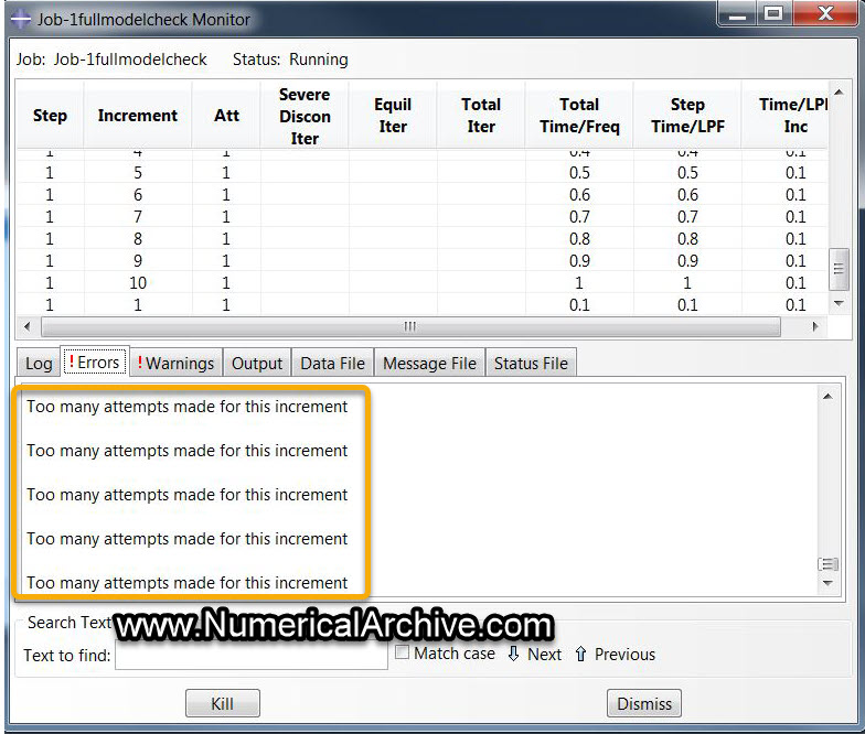
The “Too many attempts made for this increment” error is another Abaqus/Standard termination message associated with repeated failure to converge. During automatic incrementation, Abaqus can abandon a difficult increment, reduce the time increment, and attempt the state again. If the analysis repeatedly fails to establish an acceptable converged solution, the solver eventually stops.
What This Error Really Means
This message should be interpreted as persistent convergence failure in the current nonlinear state. The Newton solution process is not reaching equilibrium before the increment is abandoned. Reducing the increment may help if the original increment was simply too large, but repeated failure after cutbacks suggests a deeper modeling or response problem.
Common Causes
- Contact chattering or rapidly changing contact conditions.
- Very large plastic strain increments or severe local deformation.
- Material models with abrupt softening or poorly calibrated damage evolution.
- Unstable structural response near buckling, snap-through, or loss of load-carrying capacity.
- Inadequate constraints or rigid-body motion.
- Poor-quality elements in the critical region.
- Overly aggressive load application.
- A step procedure that is not appropriate for the physical response.
How to Fix It
Start by checking the message diagnostics and the last successful increment. If the problem is contact-driven, review contact normals, initial gaps or overclosures, master-slave or surface definitions where applicable, friction, and penalty behavior. If the failure occurs in a damaged or highly plastic region, inspect the material state and element geometry.
Smaller initial and maximum increments can improve resolution of a difficult nonlinear transition, but do not reduce them blindly. The goal is to resolve a physical transition more gradually—not to make an invalid model run for longer.
For problems involving severe post-buckling, collapse, complex contact, impact, or large deformation, reconsider the analysis procedure. A Static, General step is not always the best numerical path. Depending on the problem, a Riks procedure, Dynamic Implicit procedure, or Abaqus/Explicit analysis may be more appropriate.
Engineering note: Switching to Abaqus/Explicit does not validate the model. Explicit can continue through highly nonlinear states that Standard cannot converge through, but mesh quality, material calibration, contact behavior, energy balance, and loading rate must still be checked.
4. No Density Has Been Specified
The “No density has been specified” error is common when a model is moved from a static Abaqus/Standard workflow to Abaqus/Explicit. Mass density is required for Abaqus/Explicit materials except hydrostatic fluids, and nonzero density must be defined for non-rigid elements.
How to Fix It
- Open the Property module.
- Edit the material assigned to the affected deformable region.
- Go to General → Density.
- Enter the material density using the same consistent unit system as the rest of the model.
- Verify that the correct material and section are actually assigned to the affected region.
The unit check is critical because Abaqus does not impose a built-in unit system. A density value that is correct in SI units can be completely wrong in a millimeter-newton-tonne system or another consistent engineering unit system.
Do not enter an arbitrary density only to make the job start. Density controls inertia and influences the explicit wave speed and stable time increment. An incorrect density can change the dynamic response and can also distort the computational efficiency of an Abaqus/Explicit analysis.
5. Numerical Singularity in Abaqus
A numerical singularity warning indicates that the equation system contains a degree of freedom with extremely low or poorly defined stiffness relative to the rest of the model. In engineering terms, Abaqus may be detecting rigid-body motion, an unconstrained mechanism, disconnected regions, or a stiffness definition that is nearly singular.
Common Causes
- Missing translational or rotational restraints.
- Disconnected parts or nodes that were expected to transfer load.
- Incorrect coupling, tie, connector, or contact definitions.
- Beam or shell rotational degrees of freedom that are not properly restrained.
- Materials or sections with unrealistically small stiffness.
- Mechanisms created by hinges, releases, connectors, or geometry.
How to Diagnose It
Read the warning carefully and identify the node and degree of freedom reported by Abaqus. Display the node in the assembly and determine which physical connection should provide stiffness in that direction. Do not automatically constrain the reported node. The node may simply be the location where the solver detects a global mechanism whose true source is elsewhere.
A useful test is to review the undeformed connectivity and boundary conditions, then inspect the early deformed shape with an amplified scale factor. Unexpected rigid motion often reveals the missing connection quickly.
6. Zero Pivot Error in Abaqus
A zero pivot message is related to a singular or poorly conditioned equation system. It is often associated with insufficient constraints, redundant or conflicting constraints, disconnected degrees of freedom, or a model region that has lost effective stiffness.
The diagnostic strategy is similar to a numerical singularity warning:
- Identify the node and degree of freedom reported in the message.
- Check whether the region is connected to the load path.
- Review boundary conditions, coupling constraints, equations, MPCs, and connectors.
- Check whether damage or material degradation has reduced stiffness to a numerically problematic level.
- Inspect contact if a body relies on contact alone to prevent rigid motion.
Adding an artificial boundary condition at the reported degree of freedom may remove the error but can change the structural behavior. Restrain the physical mechanism, not the error message.
7. Excessive Distortion or Distorted Elements
Element distortion becomes critical when large deformation causes the finite element geometry to deteriorate to the point that element calculations become inaccurate or unstable. In Abaqus/Standard, severe distortion can lead to repeated cutbacks and convergence failure. In Abaqus/Explicit, highly compressed or distorted elements can reduce the stable time increment and may eventually trigger element-related termination messages.
Common Causes
- An initially poor mesh with high skewness or extreme aspect ratio.
- Insufficient mesh refinement in a localization, contact, or crushing zone.
- Abrupt mesh-size transitions.
- Incorrect contact allowing unrealistic penetration or local folding.
- Material data that produces unrealistic softening or strain localization.
- Boundary conditions that force nonphysical deformation.
- An element formulation that is poorly suited to the deformation mode.
How to Fix Distorted Elements
First identify whether the distortion is physical. Severe deformation near cutting, crushing, penetration, impact, or failure may be expected. If the distortion is nonphysical, improve the mesh topology, contact definition, material model, and boundary conditions. If the deformation is physical, consider a more suitable modeling strategy such as adaptive meshing where supported, damage with element removal when physically justified, a different element formulation, or another numerical approach appropriate to the application.
Do not use mass scaling as a cure for bad element geometry. Variable mass scaling may prevent a few compressed elements from reducing the explicit time increment, but it does not restore element quality.
8. Too Many Increments Needed or Analysis Requires an Excessive Number of Increments
An analysis can also become impractical because Abaqus requires an excessive number of increments. The interpretation depends strongly on the solver.
In Abaqus/Standard
A very large increment count often means that the solver is repeatedly reducing the increment to resolve nonlinear behavior. Review convergence history, contact changes, material state, and the location of residual or correction problems. Increasing the maximum number of increments only gives the solver permission to continue longer; it does not remove the cause of repeated cutbacks.
In Abaqus/Explicit
The total increment count is strongly influenced by the stable time increment and the total step time. A few small elements can control the entire analysis. Identify the critical elements, verify mesh necessity, and determine whether local mesh improvement, selective mass scaling, or another modeling change can remove the bottleneck.
For a detailed explanation of fixed and variable scaling, target time increments, critical elements, and energy checks, see our guide to mass scaling in Abaqus.
Abaqus Error Troubleshooting Matrix
| Error or symptom | First place to check | Common root cause | Do not do first |
|---|---|---|---|
| Missing Property Definition | Section assignments | Unassigned or invalid property region | Change solver settings |
| Time increment less than minimum | Last converged increment and diagnostics | Persistent nonlinear convergence difficulty | Set an extremely small minimum increment immediately |
| Too many attempts for increment | Message diagnostics and active nonlinear zone | Repeated failed cutbacks | Change many settings at once |
| No density specified | Material density and units | Missing density in Explicit model | Enter an arbitrary density |
| Numerical singularity | Reported node and degree of freedom | Mechanism or missing stiffness | Blindly restrain the reported node |
| Zero pivot | Constraints and connectivity | Singular or poorly conditioned system | Add artificial constraints without checking the load path |
| Excessive distortion | Critical element region | Mesh, contact, material, or physical localization | Use mass scaling as a geometry fix |
| Excessive increment count | Cutback history or explicit stable time increment | Repeated convergence difficulty or controlling small elements | Only increase the maximum increment count |
A Practical Abaqus Error Workflow
When an Abaqus job fails, use the following sequence:
- Copy the exact error message. Do not troubleshoot from memory.
- Identify Standard or Explicit. The same word “increment” has different numerical meaning in the two solvers.
- Find the failure time and increment.
- Inspect the last successful state.
- Locate the active nonlinear region.
- Review contact, mesh, material, loads, and constraints in that region.
- Check units and input magnitudes.
- Change one suspected cause.
- Rerun a short diagnostic case when possible.
- Compare the new failure state with the previous one.
A successful job is not automatically a correct model. After resolving the error, review the engineering response, energy behavior, mesh sensitivity, contact behavior, and any numerical controls introduced during troubleshooting.
Abaqus Common Errors FAQ
Why does Abaqus keep reducing the time increment?
In Abaqus/Standard, automatic incrementation reduces the increment when the nonlinear equilibrium solution is difficult or diverging. Repeated cutbacks usually indicate contact changes, severe nonlinearity, material or element calculation difficulty, instability, or another modeling problem.
Should I always reduce the minimum increment size?
No. A smaller minimum increment may allow additional attempts, but it does not correct the root cause of persistent convergence failure. Diagnose the active region and convergence history first.
Why does Abaqus/Explicit need density?
Abaqus/Explicit solves equations of motion and requires mass properties for deformable materials. Density also influences inertia, wave speed, and the explicit stable time increment.
Can switching from Standard to Explicit fix a convergence error?
It can avoid the equilibrium-iteration convergence process used by Abaqus/Standard, which is useful for some severe contact and large-deformation problems. However, changing solver does not fix incorrect material data, poor mesh, bad contact, wrong units, or unrealistic boundary conditions.
Is a completed Abaqus job necessarily correct?
No. Solver completion only means the numerical procedure reached the end of the requested step. Validation still requires engineering checks such as equilibrium, energy behavior, mesh sensitivity, material response, contact behavior, and comparison with analytical, experimental, or reference results where available.
Final Recommendation
The best way to solve an Abaqus error is to treat it as a diagnostic signal. Determine which solver is being used, identify the last successful state, locate the region responsible for the numerical difficulty, and correct the physical or numerical cause before changing global solution controls.
For Abaqus/Standard, focus on equilibrium convergence, cutbacks, contact changes, structural instability, and material or element calculation difficulties. For Abaqus/Explicit, focus on the stable time increment, critical elements, mass and energy behavior, distortion, and the physical loading rate.
A structured troubleshooting process is faster, more defensible, and more transferable to future models than trial-and-error changes. Explore the Numerical Archive model library for editable Abaqus numerical models and validated engineering simulation examples.