Choosing the right step in Abaqus is not a menu-selection problem. It is a statement about the physics you expect the finite element model to reproduce and the numerical strategy you are willing to use to obtain that response.
A static compression test, unstable postbuckling problem, low-frequency transient response, impact event, forming process, coupled thermal-stress simulation, and blast-loaded plate may all contain nonlinear material behaviour and contact. That does not mean they should use the same analysis procedure. The correct choice depends on inertia, time scale, equilibrium path, instability, contact evolution, material rate dependence, and the response quantity that will be validated.
This guide is written for researchers, postgraduate students, and engineers who need a practical method for choosing between Abaqus/Standard and Abaqus/Explicit and then selecting an appropriate analysis step. The objective is not to provide a one-line rule such as “use Explicit when Standard does not converge.” The objective is to make solver selection a traceable engineering decision.
What physical and numerical characteristics of a finite element problem should determine the Abaqus analysis procedure, and how can the selected step and solver be checked before the final model is accepted?
1. Start with the physics, not with Abaqus/Standard or Abaqus/Explicit
Before creating the first analysis step, write down the physical event being simulated. Ask whether the real problem has a meaningful time scale, whether inertia contributes to the response, whether the structure must remain in equilibrium throughout the loading history, and whether the analysis is expected to pass through instability or severe contact changes.
A useful first description is often only one sentence:
- A reinforced-concrete beam is loaded slowly until failure and the load-displacement response is required.
- A thin-walled member is followed through snap-through and postbuckling.
- A steel plate is subjected to a short-duration pressure pulse.
- A projectile impacts and penetrates a deformable target.
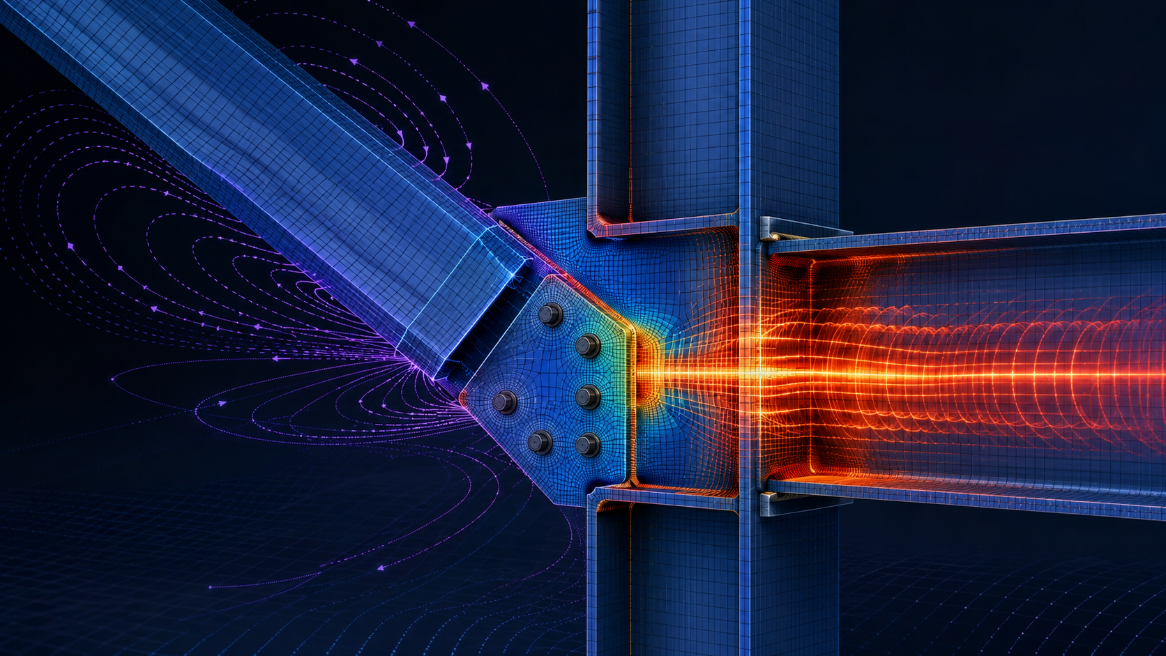
- A bolted assembly is preloaded and then subjected to service loading.
- A structural component experiences a temperature field that changes its stress response.
These descriptions are more useful than asking whether a model is “static” or “dynamic” in a casual sense. A process can be physically quasi-static but numerically difficult for an implicit solver. Abaqus/Explicit can also be used for a quasi-static objective, provided the analyst demonstrates that the accelerated numerical process has not introduced unacceptable inertial effects.
Select the procedure from the dominant physics and required response. Do not select a solver merely because a previous job converged with it.
2. What changes when you choose an analysis step?
In Abaqus/CAE, the Step module is more than a place to define loading time. The selected procedure determines which analysis product solves the problem, how equilibrium or motion is advanced, which element and interaction capabilities are available, which user subroutines can be called, and what numerical controls govern the solution.
For the structural problems discussed in this article, the two main analysis products are Abaqus/Standard and Abaqus/Explicit. Abaqus/Standard uses implicit solution procedures for general nonlinear analyses and also provides linear perturbation procedures. Abaqus/Explicit advances the solution with explicit time integration and a stability-limited time increment.
This distinction has direct consequences for:
- equilibrium iterations and convergence behaviour;
- stable time increment and the influence of very small elements;
- contact complexity and rapidly changing constraints;
- computational cost per increment and total number of increments;
- availability of specific procedures, elements, loads, and user subroutines;
- interpretation of kinetic, internal, artificial, and contact energies;
- results transfer when a simulation must move between Standard and Explicit.
3. Abaqus/Standard: an equilibrium-driven implicit solution
Abaqus/Standard is the natural starting point for many static, quasi-static, and low-speed nonlinear structural problems. In a nonlinear general step, the solver seeks equilibrium at the end of an increment and uses iterative correction when the current solution does not satisfy the equilibrium conditions.
That equilibrium-driven strategy is powerful because the increment size can be adapted and the solution can move through a long loading history without resolving every high-frequency transient. However, the procedure can become difficult when the model contains severe discontinuities, abrupt contact changes, local instability, softening, or a poorly conditioned tangent stiffness.
Typical situations where Abaqus/Standard is a strong candidate
- slowly applied structural loading where inertia is not part of the target response;
- nonlinear static analysis with plasticity, hyperelasticity, or contact that can be solved through equilibrium iterations;
- preload and service-load sequences;
- eigenvalue buckling and natural-frequency extraction;
- postbuckling problems where the Riks procedure is appropriate;
- heat transfer and many coupled or sequential multiphysics workflows;
- problems requiring Standard-specific linear perturbation procedures or other solver-specific capabilities.
Automatic incrementation is normally preferred in nonlinear static analysis because Abaqus/Standard can reduce the increment when the problem becomes difficult and increase it when the response is smooth. This is one reason a single arbitrary fixed increment is rarely a good universal strategy.
4. Abaqus/Explicit: a time-marching solution controlled by stability
Abaqus/Explicit calculates the dynamic response by advancing displacement and velocity from quantities known at the beginning of the increment. The procedure does not perform the global Newton equilibrium iterations used by a general nonlinear Abaqus/Standard step.
This makes Explicit attractive for problems involving short-duration dynamics, impact, rapidly changing contact, severe deformation, material failure, or models in which repeated implicit convergence iterations become the dominant numerical difficulty.
Typical situations where Abaqus/Explicit is a strong candidate
- impact and penetration;
- blast and short-duration pressure loading;
- crash and drop events;
- forming processes;
- large models with complicated and rapidly evolving contact;
- severe material degradation, element deletion, or extensive geometric change;
- some quasi-static problems that are prohibitively difficult to solve with equilibrium iterations.
The price of avoiding global equilibrium iterations is that explicit time integration is conditionally stable. Abaqus/Explicit automatically calculates a stable time increment. When element-by-element stability estimation controls the solution, the smallest critical element dimension and the material wave speed are central to the increment size. A few extremely small elements can therefore make an otherwise reasonable Explicit model very expensive.
Abaqus/Explicit may use inexpensive increments, but it can require a very large number of them. Computational efficiency depends on model size, stable time increment, physical event duration, contact, output frequency, and the response that must be resolved.
5. Static, General: the default choice for many slowly loaded nonlinear structures
If the target problem is a slowly applied structural load and inertia should not influence the response, Static, General is often the first procedure to evaluate.
Typical examples include a monotonic reinforced-concrete beam test, compression of a structural member, nonlinear connection analysis, or a component loaded gradually into plasticity. The procedure can include material nonlinearity, geometric nonlinearity, and contact.
Before abandoning Static, General because of a convergence error, check the model itself:
- Are the supports physically correct and sufficient to remove rigid-body motion?
- Is contact initially open, overclosed, or chattering?
- Does the material curve contain inconsistent or nonphysical data?
- Is the load applied abruptly when a smooth amplitude or smaller initial increment is required?
- Is local softening causing loss of stiffness and localisation?
- Is the model entering an unstable equilibrium path that a conventional static procedure cannot follow?
A convergence failure is evidence that the current numerical problem is difficult. It is not proof that the physics are dynamic and it is not, by itself, a reason to switch to Explicit.
6. Dynamic, Implicit: when the transient response and inertia matter
Dynamic, Implicit in Abaqus/Standard is used for nonlinear transient dynamic analysis with implicit time integration. It is appropriate when inertia and time-dependent response are important and the problem can be handled efficiently with the implicit solution strategy.
The procedure can be attractive for structural dynamics with response periods that are long compared with the very small stability-controlled increments that an explicit solution might require. The correct comparison is not simply “dynamic equals Explicit.” Both Abaqus/Standard and Abaqus/Explicit can solve dynamic problems; they use different numerical integration strategies.
When considering Dynamic, Implicit, review the time resolution required for the phenomenon, damping assumptions, contact behaviour, nonlinearities, and expected number of equilibrium iterations per increment.
7. Static, Riks: when the equilibrium path itself becomes unstable
A conventional load-controlled static analysis can struggle when the structural response passes a limit point. Examples include snap-through, snap-back-type behaviour in a selected control variable, unstable collapse, and postbuckling response.
The Static, Riks procedure follows an equilibrium path using an arc-length formulation. It should be considered when the engineering objective is to trace a nonlinear load-displacement path through instability rather than to model a rapid physical event.
This distinction is important:
Rapid physical event with important inertia → consider a dynamic procedure
Using Dynamic, Explicit only because a static model buckles can be valid for some problems, but it changes the numerical question. If the intended result is a quasi-static postbuckling equilibrium path, the analyst should compare the chosen approach with an appropriate static or arc-length solution and document the role of inertia.
8. Dynamic, Explicit for a quasi-static objective
Abaqus/Explicit is frequently used for processes that are physically quasi-static but contain severe contact, large deformation, localisation, or other nonlinearities that make an implicit solution expensive or difficult.
The central challenge is that the Explicit procedure always advances a dynamic system. The analyst therefore modifies the numerical time scale—often by applying the load faster than the real experiment—and must then demonstrate that inertial effects remain sufficiently small for the intended quasi-static interpretation.
Checks for a quasi-static Explicit analysis
- Use a smooth loading history rather than an abrupt load application.
- Review kinetic energy and internal energy throughout the important part of the response.
- Check the response for sensitivity to loading rate or total step time.
- Review mass scaling if it is used and quantify the mass change or its influence on response.
- Compare the primary engineering quantity—such as peak load or displacement—with a slower analysis where practical.
- Confirm that deformation modes are not dominated by oscillation or impact-type effects introduced by numerical acceleration.
Abaqus documentation examples commonly use the ratio of kinetic energy to internal energy as one indicator of quasi-static behaviour, but the acceptable level is problem-dependent. A single percentage should not replace engineering judgement, loading-rate sensitivity, and comparison of the final response.
9. Frequency and Buckle steps are not substitutes for nonlinear history analysis
Frequency and Buckle are linear perturbation procedures in Abaqus/Standard. They calculate a response about a base state rather than advancing the full nonlinear loading history in the same way as a general analysis step.
A frequency extraction step is useful for natural frequencies and mode shapes. An eigenvalue buckling step estimates buckling modes and critical load factors for the linearized system. These results can be extremely useful, but they should not automatically be interpreted as the nonlinear collapse load, postbuckling path, or full transient response.
For example, an eigenvalue buckling mode is often used to define an imperfection shape before a geometrically nonlinear static or Riks analysis. The perturbation result supports the nonlinear workflow; it does not replace it.
10. Thermal and coupled problems: choose the physics before the mechanical solver
When temperature affects structural response, first decide whether the thermal and mechanical fields are weakly coupled or strongly coupled.
In a sequential approach, a heat-transfer analysis may calculate the temperature field and the structural analysis then uses that temperature history as a predefined field. This can be appropriate when the mechanical response does not significantly influence the thermal solution.
In a fully coupled temperature-displacement analysis, the thermal and mechanical fields are solved together. Abaqus provides coupled procedures in both Standard and Explicit, with important differences in integration strategy and capability.
The original version of this article used the availability of DFLUX as an example of a Standard-only limitation. That statement is no longer technically defensible as a general rule: current Abaqus documentation provides DFLUX for Abaqus/Standard and VDFLUX for explicit dynamic coupled temperature-displacement analysis. Solver-specific subroutine names and interfaces must be checked against the documentation for the Abaqus release and procedure being used.
11. Element, load, interaction, and subroutine availability must be checked explicitly
Solver selection is not determined only by integration theory. A procedure may be unsuitable because a required element, load type, interaction feature, or user subroutine is not available in that analysis product or step.
Avoid statements such as “Explicit has 25 subroutines and Standard has 58.” Version-specific counts age badly and are not an engineering selection criterion. The current Abaqus documentation maintains separate Standard and Explicit user-subroutine indexes because many interfaces are solver-specific or have corresponding U/V families such as UMAT/VUMAT, DLOAD/VDLOAD, and DFLUX/VDFLUX.
Before committing a research workflow to a solver, check:
- required element formulation;
- material model availability;
- contact algorithm and interaction features;
- load and boundary-condition support;
- required output variables;
- user subroutine interface and variables passed by the solver;
- compatibility with import or results-transfer requirements.
This is especially important when a model is being migrated from an older Abaqus release or from a published paper that used version-specific features.
12. Can Abaqus/Standard and Abaqus/Explicit steps be used in the same analysis?
Implicit and explicit steps cannot be mixed in the same Abaqus analysis job. A model cannot contain a Static, General step in Abaqus/Standard followed directly by a Dynamic, Explicit step in the same job.
However, Abaqus provides results-transfer or import capabilities between analyses. A deformed mesh and associated material state can be transferred from Abaqus/Standard to Abaqus/Explicit and in supported cases from Explicit to Standard. This allows the numerical workflow to change solver when the physical stages of the problem require different procedures.
Typical Standard-to-Explicit workflow
An engineering example might apply gravity, bolt preload, or another equilibrium-controlled initial state in Standard and then continue with an impact or short-duration dynamic event in Explicit.
Typical Explicit-to-Standard workflow
Results transfer is not a magic “change solver” button. The analyst must check which elements, material states, temperatures, field variables, constraints, and model definitions are supported by the chosen transfer workflow.
13. Computational cost: why the same mesh can favour different solvers
The original article linked solver choice to upgrading computer RAM and changing seed size. Those issues may affect a real project, but they are consequences of the numerical formulation rather than useful first-order solver-selection rules.
A better way to think about computational cost is:
| Question | Abaqus/Standard | Abaqus/Explicit |
|---|---|---|
| What controls progress? | Increment size and equilibrium/convergence iterations | Stable time increment and number of explicit increments |
| What can become expensive? | Large equation systems, repeated iterations, difficult nonlinearities | Very small critical elements, long event duration, excessive output |
| Contact difficulty | Can create severe discontinuities and convergence challenges | Often attractive for rapidly changing, complex contact |
| Small local mesh | Increases model size and equation cost | Can strongly reduce the stable time increment |
| Quasi-static use | Natural when equilibrium iterations remain effective | Requires inertia and loading-rate checks |
This is why “finer mesh means more runtime” is incomplete. In Explicit, one tiny element may influence the stable time increment for the whole model. In Standard, a refined mesh increases the global system size and can also worsen local nonlinear behaviour, but the cost mechanism is different.
14. A practical decision matrix for choosing the step
| Dominant engineering problem | Procedure to evaluate first | Main validation concern |
|---|---|---|
| Slow monotonic structural loading | Static, General | Equilibrium, boundary conditions, material response |
| Unstable equilibrium path / postbuckling | Static, Riks | Path-following, imperfection sensitivity, control variables |
| Nonlinear transient with inertia | Dynamic, Implicit or Dynamic, Explicit | Time resolution, damping, contact, computational cost |
| Impact, penetration, crash, blast | Dynamic, Explicit | Time step, contact, material rate response, energy balance |
| Quasi-static but severe contact or deformation | Static, General first; Explicit may be evaluated | Loading-rate sensitivity and kinetic/internal energy |
| Natural frequencies and modes | Frequency | Base state, mass, constraints, interpretation of modes |
| Linear eigenvalue buckling estimate | Buckle | Do not interpret directly as nonlinear collapse load |
| Nonlinear postbuckling | Static, Riks or justified dynamic strategy | Imperfections, equilibrium path, inertia |
| Temperature field followed by stress response | Sequential heat transfer + stress analysis where coupling permits | Field transfer and temperature-dependent properties |
| Strong thermal-mechanical coupling | Coupled temperature-displacement procedure | Coupling assumptions and solver-specific capability |
The phrase “evaluate first” is intentional. Solver selection should be confirmed by model behaviour and validation evidence. Complex engineering models sometimes require a comparison of procedures before the final workflow is selected.
15. Common solver-selection mistakes
Using Explicit because Standard does not converge
Problem: the root cause may be an incorrect model, not the implicit solver. Check first: constraints, contact initialization, material data, load application, instability, and mesh quality.
Calling every slow experiment a Static, General problem
Problem: a physically slow test can include snap-through, severe contact, or localisation that changes the appropriate numerical strategy. Check: equilibrium path and dominant nonlinear mechanism.
Running a quasi-static problem in Explicit without energy checks
Problem: the solution can be numerically stable but physically contaminated by inertia. Check: kinetic versus internal energy, deformation mode, and loading-rate sensitivity.
Using eigenvalue buckling as the collapse load
Problem: linear perturbation buckling does not automatically capture geometric imperfection, material yielding, contact, or nonlinear postbuckling. Check: a suitable nonlinear follow-up analysis.
Ignoring the smallest elements in Explicit
Problem: a small local feature or poor mesh transition can control the stable time increment. Check: critical elements reported by Abaqus/Explicit and the reason those elements are small.
Choosing a solver before checking required subroutines
Problem: the required interface may be solver-specific or use a different U/V subroutine. Check: the current Abaqus user-subroutine index and the exact procedure.
Mixing Standard and Explicit as if they were steps in one job
Problem: implicit and explicit steps cannot be combined in one analysis job. Use: a supported results-transfer/import workflow when the physical stages require different solvers.
16. A seven-question solver selection workflow
- Does the real problem have a meaningful time scale? If yes, identify whether the time scale must be resolved in the simulation.
- Does inertia materially affect the response? If yes, use a dynamic procedure and decide whether implicit or explicit integration is more efficient.
- Must the equilibrium path be followed through instability? If yes, evaluate Riks or another justified path-following strategy.
- Is severe contact, large deformation, failure, or element deletion dominant? If yes, Explicit may offer a more practical numerical route.
- If Explicit is used for a quasi-static objective, how will inertia be ruled out? Define energy and loading-rate checks before the final job.
- Are all required elements, loads, interactions, and subroutines available in the selected procedure? Verify this in the documentation for the release being used.
- Does the problem require more than one solver stage? Plan a supported results-transfer workflow and validate the transferred state.
17. Related Numerical Archive models: two different solver-selection contexts
The purpose of presenting two different numerical models is not to declare one solver “better.” It is to show why solver selection should follow the physical event and the response that must be validated.
18. Engineering checklist before accepting the selected step and solver
- The physical event and required response quantity are defined in one clear statement.
- The importance of inertia is explicitly assessed.
- The analysis time has a physical meaning where a time-dependent procedure is used.
- Static instability is distinguished from rapid dynamic response.
- Static, General convergence problems have been investigated before changing solver.
- Riks has been considered where the equilibrium path includes a limit point or unstable postbuckling response.
- Dynamic, Implicit and Dynamic, Explicit have been compared conceptually for transient problems.
- The stable time increment and critical small elements are reviewed in Explicit.
- Quasi-static Explicit analyses include energy and loading-rate checks.
- Required elements, loads, interactions, and user subroutines are supported by the selected procedure.
- Linear perturbation results are not being interpreted as full nonlinear history results.
- Any Standard-to-Explicit or Explicit-to-Standard workflow uses supported results transfer and checks the transferred state.
- Computational cost is explained through the numerical formulation, not only by model size or computer RAM.
- The final solver choice is documented in the research report or thesis.
19. Final recommendations
The most reliable way to choose a step and solver in Abaqus is to stop asking, “Which solver is stronger?” and start asking, “What physical response must this model reproduce, and which numerical procedure advances that response with the fewest uncontrolled assumptions?”
Use Abaqus/Standard when an equilibrium-driven implicit solution matches the problem and convergence can be achieved with a physically correct model. Use Abaqus/Explicit when the problem is naturally transient or when severe contact, deformation, and rapidly changing nonlinearities make explicit time integration the more appropriate numerical strategy. Use Explicit for a quasi-static objective only when inertial effects are checked rather than assumed away. Use Riks when the equilibrium path itself is the engineering target. Use results transfer when different stages genuinely require different solvers.
The best solver choice is not the one that makes the job complete. It is the one for which the analyst can explain why the procedure matches the physics, which numerical risks were checked, and how the final response was validated.
References
- Dassault Systèmes SIMULIA — About Dynamic Analysis Procedures.
- Dassault Systèmes SIMULIA — Explicit Dynamic Analysis.
- Dassault Systèmes SIMULIA — Static Stress Analysis.
- Dassault Systèmes SIMULIA — Implicit Dynamic Analysis Using Direct Integration.
- Dassault Systèmes SIMULIA — Unstable Collapse and Postbuckling Analysis.
- Dassault Systèmes SIMULIA — Multiple Step Analysis.
- Dassault Systèmes SIMULIA — About Transferring Results between Abaqus Analyses.
- Dassault Systèmes SIMULIA — User Subroutine Functions Listing.
- Dassault Systèmes SIMULIA — Thermal Loads, including DFLUX and VDFLUX.