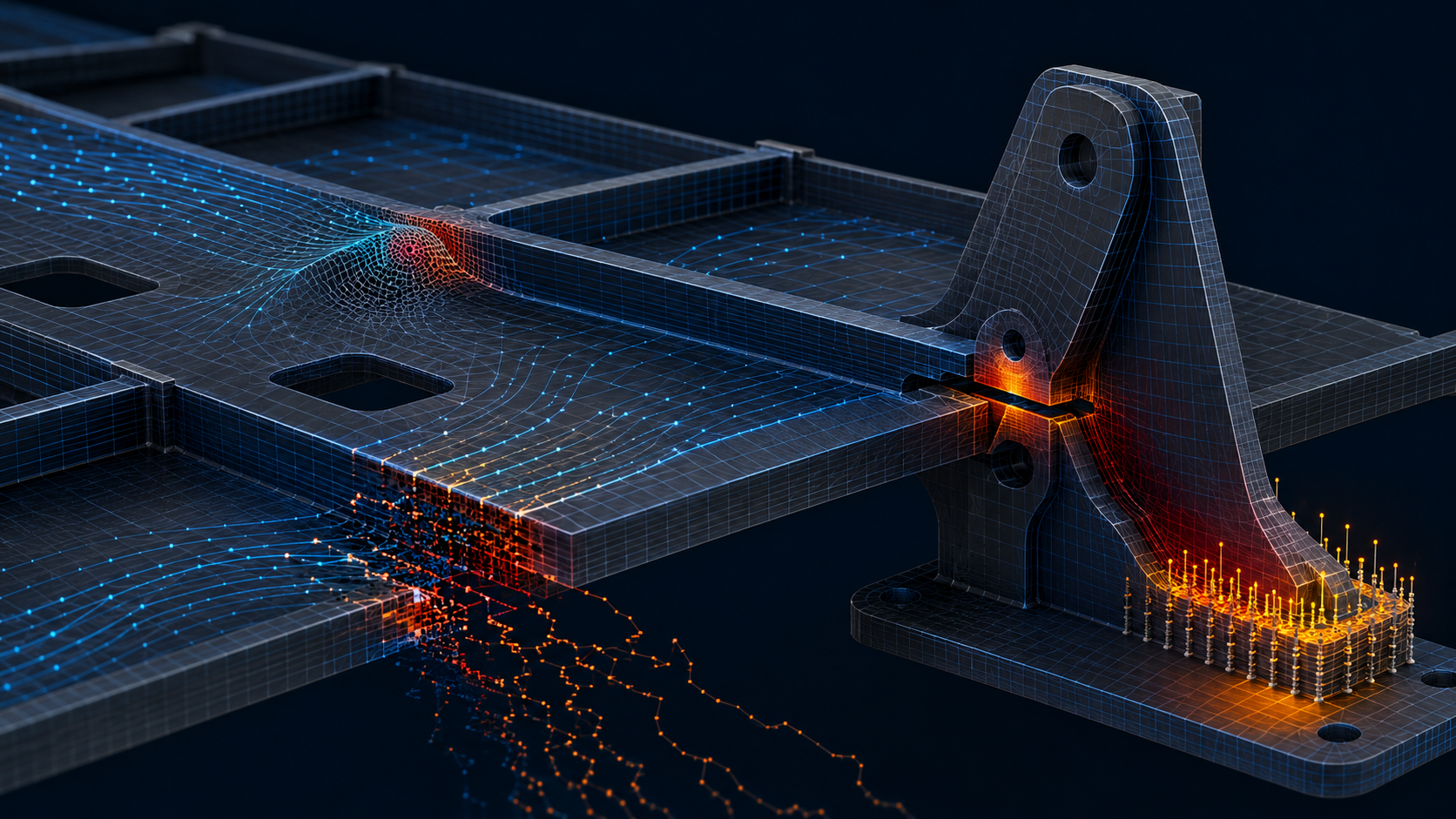
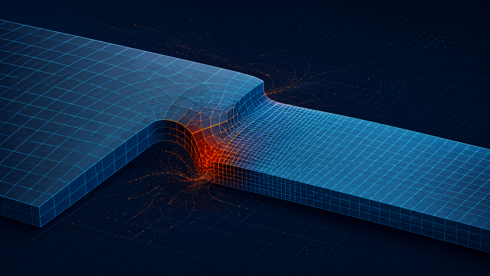
Distorted Elements in Abaqus: Causes and Fixes

Distorted elements in Abaqus are not a single error with a single fix. The same warning can be caused by an initially poor mesh, extreme material deformation, contact penetration, an unsuitable element formulation, incorrect material data, an unrealistic loading history, or a physical failure mechanism that the chosen Lagrangian mesh can no longer represent.

The correct troubleshooting question is therefore not simply “How do I remove the distorted element error?” The better question is: why is this element changing shape so severely, and is that deformation physical or numerical?

This guide explains how to diagnose excessive element distortion in Abaqus/Standard and Abaqus/Explicit, how distortion affects convergence and the explicit stable time increment, and when to use mesh improvement, a different element formulation, contact corrections, ALE adaptive meshing, damage with element deletion, or another analysis strategy.

Engineering note: Never treat “the job completed” as proof that the distortion problem was solved correctly. A numerical control can keep an analysis running while the underlying model remains physically wrong. Always review the deformed mesh, material response, contact behavior, energy history, and sensitivity of the engineering outputs.

What Is Element Distortion in Abaqus?

Finite elements map an ideal parent element to the actual element geometry in the model. As the analysis proceeds, the nodal coordinates change and the element geometry changes with them. Moderate distortion is normal in a large-deformation analysis. The problem begins when the element shape becomes so poor that strain calculation, stress integration, contact treatment, or the numerical solution becomes inaccurate or unstable.

Examples include a brick element becoming extremely flat, a quadrilateral becoming severely skewed, a solid element approaching zero volume, or a localized band of elements stretching and collapsing under damage. In severe cases, an element can invert or develop a nonphysical geometry.

It is important to distinguish two situations:

Poor initial element quality: the element is already badly shaped before the analysis starts.
Evolving element distortion: the initial mesh is acceptable, but the element becomes severely distorted as the solution evolves.

These situations require different fixes. Initial mesh problems should usually be corrected before the analysis. Evolving distortion requires investigation of the deformation mechanism, element formulation, material law, contact, and numerical procedure.

Why Distorted Elements Are a Serious Problem

Excessive distortion can affect an Abaqus model in several ways.

Loss of Result Accuracy

Element interpolation and numerical integration are most reliable when the element geometry remains within the range expected by the formulation. Severe skewness, flattening, warping, or collapse can degrade the calculation of strains and stresses. Local contour values may become dominated by mesh pathology rather than the physical response.

Convergence Failure in Abaqus/Standard

In Abaqus/Standard, strongly distorted elements can contribute to severe nonlinear behavior and element calculation difficulties. The solver may repeatedly reduce the time increment, fail to establish equilibrium, and terminate with messages such as “Time increment required is less than the minimum specified” or “Too many attempts made for this increment.”

For a broader convergence diagnostic workflow, see Abaqus common errors and practical fixes.

Reduction of the Stable Time Increment in Abaqus/Explicit

In Abaqus/Explicit, the stable time increment is strongly related to element characteristic length and dilatational wave speed. When an element becomes highly compressed or its characteristic dimension becomes very small, the element can reduce the stable time increment and increase the total number of increments required to complete the step.

This is why a job may begin with an acceptable computational speed and then become progressively slower during crushing, impact, penetration, or severe forming. A small group of highly deformed elements can become the time-increment-controlling region.

Mass scaling can improve explicit efficiency when a limited group of elements controls the stable time increment, but mass scaling does not repair element geometry. Read our detailed guide to mass scaling in Abaqus before using it as part of an explicit troubleshooting strategy.

First Question: Is the Distortion Physical or Numerical?

Before changing the mesh, decide whether the deformation itself is expected.

Physical extreme deformation may occur in:

metal forming and extrusion;
crushing and compaction;
cutting and machining;
penetration and high-speed impact;
concrete crushing or localized damage;
soil or soft-material flow;
rubber and highly deformable materials;
fracture zones and material separation.

If the material is physically expected to undergo extreme shape change, repeatedly refining a purely Lagrangian mesh may only delay the distortion. The analysis strategy itself may need to change.

By contrast, nonphysical distortion often appears because of:

incorrect material parameters;
wrong units;
contact penetration or bad contact geometry;
unrealistic boundary conditions;
an abrupt load application;
poor initial mesh topology;
a tiny sliver element;
an unsuitable element formulation;
damage localization without an objective regularization strategy.

Do not solve a numerical distortion problem with a physical failure mechanism, and do not suppress a real physical deformation only to make the mesh look better.

How to Identify Distorted Elements in Abaqus

The fastest troubleshooting workflow is to locate the exact elements, identify when they begin to deteriorate, and compare that time with the evolution of material, contact, and loading variables.

1. Read the Warning and Error Messages

Record the exact Abaqus message. Do not troubleshoot from memory. Determine whether the job reports excessive distortion, negative volume, element calculation problems, convergence cutbacks, deformation speed warnings, or a rapidly decreasing stable time increment.

Also record the step, increment, and analysis time associated with the failure. In Abaqus/Standard, review the message diagnostics and convergence history. In Abaqus/Explicit, review the status and diagnostic information and identify critical elements when stable-time-increment behavior is involved.

2. Inspect the Last Valid Frames

Do not inspect only the final frame. Move backward several output frames and watch the distortion develop. Ask:

Does the element collapse suddenly or gradually?
Does distortion start when contact is established?
Does it begin when material damage activates?
Is the distorted region associated with a stress or strain localization band?
Does the mesh fold because of a boundary condition?
Is the deformation concentrated around one poor element?

A short animation of the deformed mesh is often more informative than a single stress contour.

3. Display Element Labels and Create a Diagnostic Set

Identify the problematic element labels and create an element set for troubleshooting. Once the region is isolated, inspect local geometry, mesh size, section assignments, material definitions, contact participation, and history output.

For a large model, this is more efficient than changing global controls. Most severe distortion problems are local even when they eventually terminate the entire job.

4. Check the Initial Mesh Quality

Verify the mesh before running the model. Look for poor aspect ratio, excessive skewness, severe warpage, small angles, abrupt transitions, and tiny elements created by short geometric edges or partitions.

A common mistake is to assume that a finer mesh is always safer. One accidentally tiny element can create a local distortion problem and can also control the Abaqus/Explicit stable time increment.

Main Causes of Distorted Elements in Abaqus

1. Poor Mesh Topology or Bad Initial Element Shape

An element that begins with poor geometry has less capacity to accommodate additional deformation. Highly skewed or flattened elements can become unusable after a relatively small shape change.

Typical causes include:

automatic meshing around small geometric features;
sliver faces and short edges;
poor partitioning;
abrupt mesh-density transitions;
high-aspect-ratio elements in the wrong deformation direction;
unstructured mesh topology in a highly localized deformation zone.

The correct fix is often geometric cleanup and repartitioning, not simply reducing the global seed size.

2. Insufficient Local Mesh Resolution

A coarse element may be forced to represent a steep strain gradient, sharp curvature, bending localization, crushing zone, or contact-pressure gradient. The element then undergoes a large change in shape over a small number of degrees of freedom.

Use targeted refinement in the physical deformation zone and maintain a smooth transition to the surrounding mesh. Avoid refining the entire model unless the response requires it.

In Abaqus/Explicit, remember that refinement increases element count and can reduce the stable time increment. Refinement must therefore be justified by both accuracy and computational sensitivity.

3. Incorrect Element Type or Formulation

There is no universal rule that “quadratic elements fix distortion” or that “full integration is always better.” The correct element depends on the deformation mode, material behavior, incompressibility, bending response, contact, and solver.

Review:

continuum versus shell representation;
linear versus higher-order interpolation;
reduced versus full integration;
hourglass behavior in reduced-integration elements;
locking behavior;
formulations appropriate for nearly incompressible material behavior;
element suitability for severe deformation and contact.

Changing element type can move the numerical problem rather than solve it. Compare the deformation pattern and response with a reference formulation whenever possible.

4. Unrealistic Material Behavior

Many distorted-element failures are material-model failures disguised as mesh failures.

Check for:

wrong modulus, yield stress, density, or strain units;
unrealistically low stiffness;
abrupt post-peak softening;
damage evolution that localizes into one element row;
incorrect plastic data ordering;
nearly incompressible response with an unsuitable formulation;
hyperelastic parameters outside the calibrated strain range;
concrete damage parameters that produce uncontrolled local degradation.

Plot stress-strain behavior from the material definition independently of the full model. If the constitutive response is physically unreasonable, mesh changes will not produce a reliable analysis.

5. Contact-Induced Element Distortion

Contact can create highly localized forces and deformation. Distortion near an interface should trigger a detailed review of:

initial overclosure or penetration;
surface normals and surface selection;
sharp rigid edges contacting a coarse deformable mesh;
friction and tangential behavior;
contact stiffness and penalty effects;
self-contact where large folding occurs;
overconstraints caused by combining contact, ties, coupling, and boundary conditions.

Watch the contact region immediately before distortion starts. If one element is trapped, penetrated, or folded by an interface, refining an unrelated area will not help.

6. Loading and Boundary-Condition Problems

An unrealistic load amplitude, abrupt prescribed displacement, incorrect load direction, or incompatible boundary condition can force the mesh into a nonphysical deformation mode.

For dynamic and explicit analyses, an abrupt load can generate stress waves and local transient deformation. For quasi-static explicit simulations, apply the loading smoothly and verify that kinetic energy remains appropriately small relative to the structural response.

For Abaqus/Standard, a sudden nonlinear transition can produce repeated cutbacks and convergence failure. The solution may require a more suitable load history or analysis procedure rather than an arbitrary minimum increment change.

7. Physical Localization, Damage, and Failure

A model may distort because the simulated material is actually failing. Cracking, crushing, shear banding, necking, and ductile fracture can concentrate deformation into a narrow region.

In this case, the question is whether the finite element model has an appropriate method to represent post-localization behavior. Possible considerations include mesh-objective damage regularization, characteristic-length-based damage evolution, physically calibrated failure criteria, and element deletion when loss of load-carrying capacity and material separation are part of the intended model.

Element deletion is not a cosmetic mesh-cleaning tool. Deleting elements changes mass, energy, contact surfaces, and load paths. Use it only when supported by the physical failure model and verify the energy and response sensitivity.

How to Fix Distorted Elements in Abaqus

1. Fix Poor Mesh Geometry First

If the problematic element is initially poor, repair the geometry and mesh topology before changing solver controls.

Locate the element and its neighboring elements.
Inspect short edges, sliver faces, and partition intersections.
Repartition the region to create a structured or more regular mesh where practical.
Use local seeds rather than extreme global refinement.
Create a smooth mesh-size transition.
Rerun the mesh verification checks.

For Abaqus/Explicit, also compare the minimum stable time increment before and after the mesh change. Removing one tiny element can provide a larger efficiency improvement than mass scaling the entire model.

2. Refine Only the Physical Deformation Zone

Refinement is appropriate when the physical strain or curvature gradient is not adequately resolved. Refine the contact patch, notch, crushing region, bending zone, or localization area—not every part in the model.

Then perform a mesh sensitivity study using the engineering quantity that matters: force-displacement response, energy absorption, crack path, reaction force, peak displacement, penetration depth, or another problem-specific metric.

3. Review the Element Formulation

Select the formulation based on the dominant physics. For a thin structure undergoing bending, a shell representation may be more appropriate than a few poorly shaped continuum elements through the thickness. For nearly incompressible behavior, use a formulation appropriate to that response. For reduced-integration elements, monitor hourglass-related artificial energy and deformation modes.

Do not switch all elements blindly. Create a controlled comparison model and review both deformation and the target engineering output.

When distortion begins at contact, inspect the contact mechanics before refining repeatedly. Improve the surface discretization, verify initial clearances, check interaction properties, and make sure the deformable surface has sufficient local resolution to represent the contact pressure and curvature.

If a sharp rigid feature is physically correct, the deformable mesh may need local refinement or a different modeling strategy. If the sharp feature is a CAD artifact that has no engineering significance, geometric simplification may be the better fix.

5. Correct Material and Damage Input

Verify the full material response over the strain range reached by the analysis. For tabular plasticity, damage, hyperelasticity, or rate-dependent data, check the units and ordering of every input column.

For damage models, compare the initiation and evolution parameters with the characteristic element size and the calibration basis. If the result changes dramatically with mesh size, the observed distortion may be part of a mesh-dependent localization problem.

6. Use a Physically Appropriate Loading History

Apply loads and prescribed displacements smoothly when the physical event is gradual. Avoid numerical shocks created by an abrupt amplitude unless the real event is itself impulsive.

In quasi-static Abaqus/Explicit analysis, compare kinetic energy with internal energy and review the force-displacement response. Slowing the loading may reduce inertial contamination, although it increases computational cost.

7. Consider Distortion Control in Abaqus/Explicit

For supported solid-element applications in Abaqus/Explicit, distortion control can be used to resist excessive element deformation. It should be treated as a numerical control with a specific purpose, not a universal switch for every distorted mesh.

Distortion control can introduce additional numerical resistance to deformation. Therefore, verify that it does not artificially stiffen the response or change the failure mechanism. Compare reaction forces, deformation, and energy histories with a reference case.

8. Use ALE Adaptive Meshing for Suitable Large-Deformation Problems

Arbitrary Lagrangian-Eulerian adaptive meshing can improve mesh quality by allowing the mesh motion to differ from the material motion. This can be valuable in large-deformation problems where the Lagrangian mesh progressively deteriorates but the material topology does not require arbitrary separation.

ALE adaptive meshing is not equivalent to simply generating a new mesh after every increment. Its suitability depends on the element types, procedure, material behavior, contact, and physical problem. Validate advection and state-variable behavior for the quantities important to the study.

9. Consider Eulerian or CEL Methods for Extreme Material Flow

If the material undergoes deformation so extreme that a Lagrangian mesh cannot reasonably follow it, an Eulerian or coupled Eulerian-Lagrangian strategy may be more appropriate. Penetration, fluid-like material flow, severe impact, and some explosion problems are typical examples where mesh motion must be separated from material motion.

Changing to CEL is a modeling-strategy decision, not a quick error fix. Contact, material volume fractions, boundary conditions, output interpretation, and computational cost all require a different workflow.

10. Use Damage and Element Deletion Only When Failure Is Physical

If the physical material loses load-carrying capacity and separates, damage evolution with element deletion can prevent failed elements from continuing to deform indefinitely. However, the failure criterion and evolution law must be calibrated.

After enabling deletion, review:

mesh sensitivity of the failure pattern;
energy dissipation;
mass loss;
contact changes after deletion;
reaction force or impact-force sensitivity;
the physical timing of failure.

Why Mass Scaling Does Not Fix Distorted Elements

This confusion is common in Abaqus/Explicit. As elements compress and their characteristic length decreases, the stable time increment may decrease. Variable mass scaling can increase the stable time increment and prevent the computational cost from growing as rapidly.

But the element may still be badly distorted.

Mass scaling changes mass and inertia. It does not improve the Jacobian mapping, restore element shape, correct contact penetration, repair an incorrect material model, or remove a sliver element. If distortion is the root problem, mass scaling can hide the computational symptom while the mesh continues to deteriorate.

Use mass scaling in Abaqus only after the controlling elements and deformation mechanism are understood.

Distorted Elements in Abaqus/Standard vs Abaqus/Explicit

Issue	Abaqus/Standard	Abaqus/Explicit
Primary numerical symptom	Convergence difficulty, cutbacks, element calculation problems	Decreasing stable time increment, extreme deformation, possible termination
First diagnostic focus	Last converged increment and nonlinear convergence history	Critical elements, deformation history, stable time increment, energies
Common local causes	Contact changes, instability, material softening, mesh distortion	Compression, impact, contact, severe deformation, material flow
Does a smaller increment fix geometry?	No	No
Can mass scaling help?	Not as a Standard convergence control	It can improve efficiency but does not repair distortion
Alternative strategies	Mesh/material/contact correction, suitable procedure such as Riks or Explicit	Mesh correction, distortion control, ALE, damage/deletion, Eulerian or CEL where appropriate

A Practical Distorted-Element Diagnostic Workflow

Copy the exact Abaqus warning or error.
Identify the solver: Standard or Explicit.
Record the failure step, increment, and time.
Locate the exact distorted elements.
Move backward through several output frames.
Determine when the element shape begins to deteriorate.
Check contact, material state, loads, and boundary conditions at that time.
Verify the initial mesh quality and local geometry.
Decide whether the distortion is physical or numerical.
Apply the smallest targeted modeling change.
Rerun and compare the deformation history.
Perform a sensitivity check on the engineering output.

Best practice: Save a diagnostic copy of the model before every major change. If you change mesh, contact, material, loading, and step controls simultaneously, a successful rerun will not tell you which change solved the problem.

Distorted Elements Troubleshooting Matrix

Observed behavior	Likely first suspect	First action
One poor element distorts immediately	Initial mesh or sliver geometry	Inspect local topology and remesh
Distortion begins at first contact	Contact geometry or penetration	Review surfaces, clearances, and local mesh
Distortion begins when damage activates	Material softening or localization	Review damage calibration and mesh sensitivity
Explicit job becomes progressively slower	Compressed controlling elements	Review critical elements and stable time increment
Elements fold under prescribed displacement	Boundary condition or load path	Review kinematics and deformation mode
Rubber-like material develops poor response	Material/formulation suitability	Review compressibility and element formulation
Physical material flow destroys Lagrangian mesh	Analysis strategy limitation	Evaluate ALE, Eulerian, or CEL methods
Deleted region changes force response dramatically	Failure/deletion calibration	Review energy, mesh sensitivity, and failure law

Distorted Elements in Abaqus FAQ

What causes distorted elements in Abaqus?

Common causes include poor initial mesh quality, severe physical deformation, incorrect material data, contact penetration, unsuitable element formulation, abrupt loading, damage localization, and boundary-condition problems.

Should I always refine the mesh to fix distorted elements?

No. Targeted refinement can help when a physical deformation gradient is under-resolved, but global refinement can increase computational cost and may create smaller time-increment-controlling elements in Abaqus/Explicit. Fix mesh topology, geometry, contact, and material problems first.

Can I use mass scaling to remove excessive distortion?

No. Mass scaling can increase the explicit stable time increment, but it does not restore element geometry. Use mass scaling only for a justified computational bottleneck after diagnosing the distortion mechanism.

Does switching from Abaqus/Standard to Abaqus/Explicit fix distorted elements?

Not automatically. Explicit avoids the equilibrium-iteration convergence process used by Standard and can be effective for severe contact and large deformation, but an incorrect mesh, material model, contact definition, or boundary condition remains incorrect.

When should I use ALE adaptive meshing?

Consider ALE adaptive meshing when large deformation progressively damages a Lagrangian mesh and the problem is compatible with the supported adaptive-meshing capabilities. Validate the response and state-variable transport for the engineering outputs of interest.

Should I delete distorted elements?

Only when element deletion represents a physically calibrated loss of load-carrying capacity or material separation. Deleting elements simply because they distort can create nonphysical mass, energy, contact, and load-path changes.

How do distorted elements affect the Abaqus/Explicit stable time increment?

As an element becomes compressed or its characteristic dimension decreases, its stable time increment can decrease. A few highly deformed elements may then control the computational cost of the entire explicit model.

Final Engineering Recommendation

The most reliable way to fix distorted elements in Abaqus is to diagnose the deformation mechanism before changing numerical controls. Locate the exact elements, identify the first time at which their shape begins to deteriorate, and compare that event with contact, material state, loading, and boundary-condition changes.

If the initial mesh is poor, repair the mesh. If contact is forcing local collapse, correct the contact model. If material softening is localizing into one element row, review the constitutive and damage formulation. If the physical problem involves extreme material flow, consider ALE, Eulerian, or CEL strategies. If elements are physically failing, use a calibrated damage and deletion model rather than deleting them merely to keep the job running.

Abaqus provides several tools that can help severe-deformation analyses, but no single switch replaces engineering diagnosis. The correct solution is the one that removes the numerical pathology while preserving the physical response and the conclusions of the simulation.

Explore the Numerical Archive Abaqus model library for editable finite element models and validated engineering simulation examples.

Distorted Elements in Abaqus: Causes, Diagnosis, and Practical Fixes