Mass Scaling in ABAQUS

Mass scaling in Abaqus is one of the most useful—and most frequently misused—tools in Abaqus/Explicit. The idea is simple: a limited increase in element mass can increase the stable time increment and reduce the number of increments required to complete an explicit analysis. The engineering challenge is to gain computational speed without allowing the artificial change in mass and inertia to alter the response that you are trying to simulate.

This guide explains mass scaling in Abaqus/Explicit from a practical engineering point of view. It covers the stable time increment, controlling elements, fixed and variable mass scaling, target time increment selection, quasi-static and dynamic analyses, energy checks, and the diagnostics that should be reviewed before accepting a mass-scaled result.

Engineering note: Mass scaling is not a substitute for a poor mesh, an incorrect material model, or an inappropriate analysis procedure. Use it after identifying why the explicit stable time increment is small and after deciding that the added mass will not materially change the response of interest.

What Is Mass Scaling in Abaqus?

In Abaqus/Explicit, mass scaling is a numerical technique that modifies the mass of selected elements—or, in some cases, the entire model—to improve computational efficiency. It is used most commonly in quasi-static explicit analyses and in dynamic analyses where a small number of very small elements control the stable time increment.

Abaqus/Explicit integrates the equations of motion using an explicit central-difference scheme. The method advances the solution through many small increments and does not use the equilibrium iterations associated with an implicit procedure. The cost of this approach depends strongly on the stable time increment. If a few elements force the analysis to use an extremely small increment, the entire model can become computationally expensive.

Mass scaling addresses that problem by increasing mass where appropriate. The increase in mass can raise the stable time increment, reduce the number of increments, and shorten the analysis time. The benefit is real, but so is the numerical consequence: mass and inertia are physical properties. Therefore, the scaled model must be checked to confirm that its response remains representative of the intended problem.

Why Small Elements Control the Stable Time Increment

A useful engineering interpretation of the explicit stability limit is the time required for a dilatational wave to travel across an element. In simplified form:

Δtstable ≈ Lchar / cd

where Lchar is a characteristic element length and cd is the dilatational wave speed. This relationship immediately explains why one tiny element can slow a large model: reducing the controlling element length reduces the stable time increment.

Element size is not the only factor. Material stiffness, density, element formulation, contact stiffness, damping, and changes in geometry during large deformation can also influence the stability limit. In a model with several materials, an element associated with a high wave speed may control the initial time increment even when the mesh is relatively uniform.

Before applying mass scaling, perform a data check or inspect the explicit diagnostic information. The Abaqus status file can report the estimated minimum stable time increment and list elements with the smallest stable time increments. Abaqus/Explicit can also write critical elements and their stable time increments to the output database for visualization.

Practical rule: first locate the controlling elements. Then ask why they are controlling the analysis. A small sliver element created by poor partitioning should usually be fixed. A deliberately refined impact zone may justify selective mass scaling.

How Mass Scaling Increases the Stable Time Increment

The wave speed used in the explicit stability estimate depends on material stiffness and density. Increasing the mass density of an element reduces its wave speed and can increase its stable time increment. Abaqus mass scaling uses this relationship in a controlled way without requiring you to manually redefine the physical material density.

This is why mass scaling can be very effective when only a small group of elements controls the step. If the masses of those controlling elements are adjusted, the minimum element-by-element stable time increment may increase significantly while the total mass properties of the model change only slightly.

The same logic also explains the main danger. If mass is added too aggressively or over a large region, inertial forces can change. A model intended to represent a quasi-static process may become artificially dynamic, and a truly dynamic simulation may develop an incorrect transient response.

Fixed vs Variable Mass Scaling in Abaqus

Abaqus/Explicit provides two main forms of element mass scaling: fixed mass scaling and variable mass scaling. They can be used separately or together, and they can be applied globally or to selected element sets.

Fixed Mass Scaling

Fixed mass scaling is applied once at the beginning of the step in which it is defined. You can specify a mass scaling factor directly or define a desired minimum element-by-element stable time increment and allow Abaqus/Explicit to calculate the required scaling factors.

Fixed mass scaling is particularly useful when the source of the small stable time increment exists at the beginning of the analysis. Typical examples include a few small elements created by local mesh refinement or a small geometric feature that cannot reasonably be removed from the model.

Because the scaling operation occurs only once at the beginning of the step, fixed mass scaling is computationally efficient and easy to interpret.

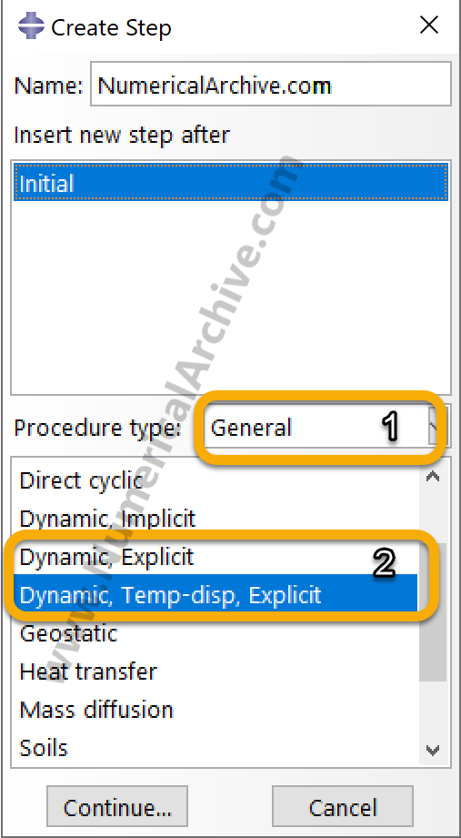
In Abaqus/CAE, create a Dynamic, Explicit step and open the Mass Scaling settings for the step.

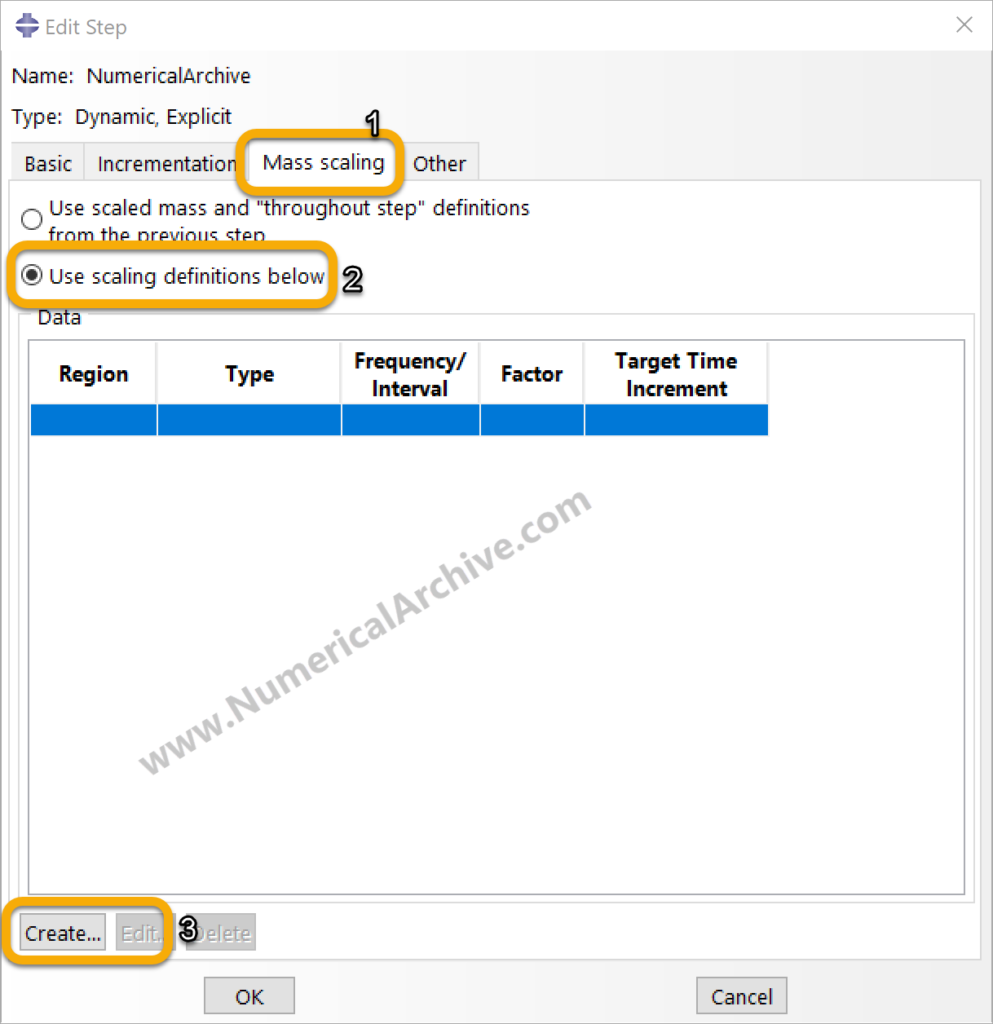
Select the option to use a mass scaling definition and create a semi-automatic mass scaling entry.

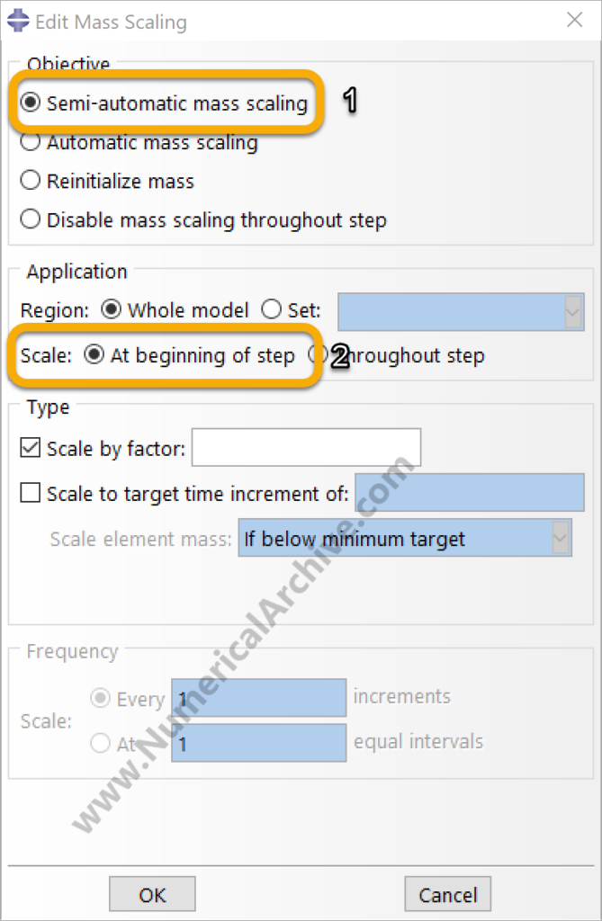
For fixed mass scaling, choose At beginning of step. The definition can then be based on a direct scale factor or on a target stable time increment, depending on the engineering objective.

Variable Mass Scaling

Variable mass scaling can be applied at the beginning of the step and periodically during the step. You define a desired minimum stable time increment, and Abaqus/Explicit recalculates and applies mass scaling factors as required.

This is useful when the elements controlling the stable time increment change during the analysis. Large compression, crushing, forming, impact, and severe deformation can reduce element characteristic lengths as the step progresses. A model that begins with a reasonable stable time increment may become much slower later in the analysis.

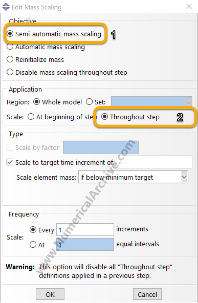
For variable mass scaling in Abaqus/CAE, select Throughout step. Do not use this option as an automatic cure for every decreasing time increment. First determine whether the reduction is a reasonable consequence of the physics or a symptom of excessive distortion, contact problems, or a poor mesh.

Mass Scaling in Quasi-Static Abaqus Explicit Analysis

Abaqus/Explicit is frequently used for quasi-static problems involving severe contact, complex nonlinearities, forming, collapse, or other situations in which an implicit solution may be difficult. For rate-independent material behavior, the natural physical time scale is generally less important than it is in a transient dynamic event.

This creates an opportunity to improve computational efficiency by reducing the step time, increasing the mass, or using a combination of careful loading and mass scaling. The objective is to obtain the required equilibrium path while keeping inertial effects sufficiently small.

For a quasi-static analysis, mass scaling should be judged from the response of the model—not from a single mass scaling factor. Review the energy history, reaction forces, displacements, stresses, plastic strains, contact response, and any other quantities that define the engineering conclusion.

A particularly important energy check is the relationship between kinetic energy and internal energy. In a quasi-static explicit analysis, ALLKE should remain a small fraction of ALLIE. Do not convert this statement into a universal percentage rule for every model. Loading history, local instabilities, contact events, and the response quantity of interest must all be considered.

Recommended workflow: run a conservative baseline or a lower-scaling case, record the engineering outputs that matter, increase the scaling in stages, and compare the results. The acceptable mass scaling level is the level at which the conclusions remain insensitive to the numerical acceleration.

Mass Scaling in Dynamic and Impact Problems

Mass scaling requires more caution in a truly dynamic analysis because the physical mass and inertia directly influence acceleration, momentum transfer, wave propagation, impact forces, and transient response.

However, a dynamic model may contain only a few very small elements that control the stable time increment. If those elements represent a negligible portion of the total mass and do not dominate the response of interest, selective mass scaling can significantly improve efficiency with a small effect on the overall dynamic behavior.

Impact simulations are a common example. Elements near an impact zone can become highly compressed and their characteristic lengths can decrease during the analysis. Variable mass scaling applied to a limited region can prevent a few severely compressed elements from reducing the time increment for the entire model.

The word limited is important. Global aggressive mass scaling in a transient dynamic model can change the physics. Compare acceleration, velocity, contact force, momentum-related response, energy histories, and other event-specific outputs against a less-scaled reference solution.

How to Identify Time-Increment-Controlling Elements

Do not guess which elements control the stable time increment. Abaqus/Explicit provides diagnostic information for this purpose.

1. Run a data check or the initial analysis setup.
2. Open the .sta status file and review the stable time increment report.
3. Identify the elements with the smallest reported stable time increments.
4. Visualize the critical elements in Abaqus/CAE when diagnostic output is available.
5. Check their geometry, characteristic length, material, section assignment, contact participation, and deformation history.

A small number of controlling elements usually suggests a local problem or a local opportunity for mass scaling. A large population of controlling elements may indicate that the entire mesh, material wave speed, or analysis strategy is responsible for the computational cost.

Before mass scaling, ask these questions:

• Is the element small because of an accidental sliver or poor partition?
• Is the local mesh finer than the physics requires?
• Does the element use the intended material and density?
• Is high contact penalty stiffness reducing the time increment?
• Is severe distortion reducing the element characteristic length during the step?
• Would local remeshing or a smoother mesh transition solve the problem more honestly?

If the answer reveals a modeling error, fix the model. If the small element is intentional and its added mass can be shown to have negligible influence, mass scaling becomes a defensible numerical strategy.

How to Choose a Target Time Increment

There is no universal target time increment that is correct for every Abaqus/Explicit model. The target should come from the distribution of stable time increments in your model and from sensitivity checks.

A practical engineering approach is:

1. Record the current minimum stable time increment.
2. Identify the elements controlling that minimum.
3. Compare their stable time increments with the larger population of elements.
4. Choose a moderate target that removes the isolated numerical bottleneck rather than forcing the entire model to an arbitrary large increment.
5. Apply mass scaling locally when possible.
6. Run the analysis and review the mass scaling and energy outputs.
7. Repeat with a lower target or a no-scaling reference and compare the engineering response.

If one tiny element has a stable time increment orders of magnitude below the rest of the model, targeting that isolated bottleneck may provide a large computational benefit. If many important structural elements require substantial added mass to reach the chosen target, the target is probably too aggressive or the analysis strategy should be reconsidered.

Defining a Mass Scaling Factor Directly

A direct scale factor is a fixed mass scaling method. The specified factor is applied to the original masses of the selected elements at the beginning of the step. This method is simple and transparent, but the user is responsible for understanding how the selected factor changes the mass properties of the model.

The Abaqus/CAE path is:

Step module → Create Step → Dynamic, Explicit → Mass scaling → Use scaling definitions below → Create → Semi-automatic mass scaling → At beginning of step → Scale by factor

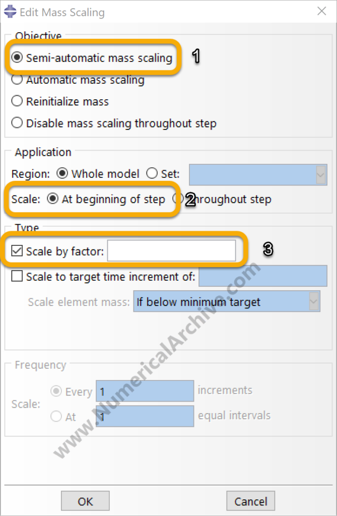
For quasi-static work, the energy history and sensitivity of the structural response must still be checked. A direct scale factor should not be selected simply because it reduces the runtime.

Target Element-by-Element Stable Time Increment

Instead of entering a scale factor directly, you can define a desired element-by-element stable time increment. Abaqus/Explicit then determines the required mass scaling factors.

The explicit solver initially evaluates the stability limit on an element-by-element basis. A global stability estimator may later provide a larger time increment when its use is appropriate. Therefore, the actual time increment used by the analysis does not necessarily equal the target value entered in the mass scaling definition.

This point is especially important when mass scaling is applied to only part of the model. Unscaled elements can still have smaller stable time increments and continue to control the element-by-element estimate.

Penalty contact can also influence the time increment. If contact stiffness is responsible for the reduction, investigate the contact formulation and contact diagnostics rather than assuming that element mass scaling is the only solution.

Uniform Mass Scaling

With uniform mass scaling based on a target time increment, Abaqus/Explicit applies one scaling factor to all elements in the selected region so that the minimum element stable time increment in that region reaches the specified target.

This approach can be useful in quasi-static analyses where a uniform adjustment is acceptable and kinetic energy remains small. The mass scaling factor is determined by Abaqus rather than entered directly by the user.

The Abaqus/CAE path is:

Step module → Create Step → Dynamic, Explicit → Mass scaling → Create → Semi-automatic mass scaling → At beginning of step or Throughout step → Scale to target time increment → Uniformly to satisfy target

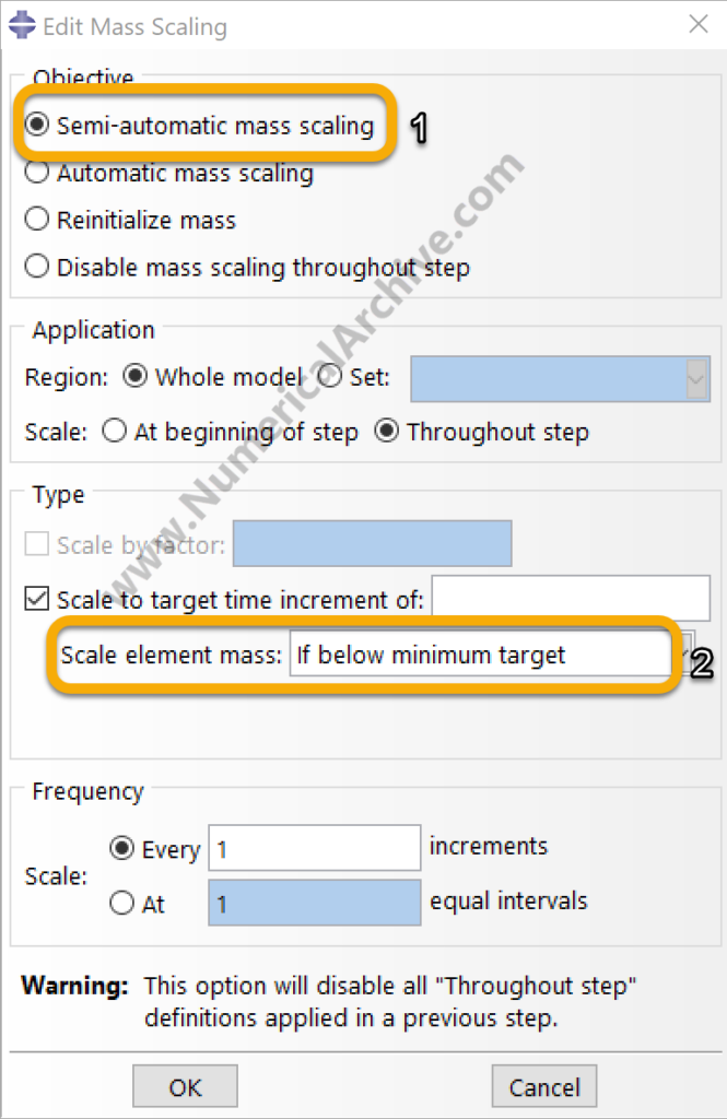
Uniform scaling is not automatically safer than local scaling. If only a few elements are causing the problem, scaling a broad region can add unnecessary mass. Always match the scaling region to the numerical bottleneck.

Local vs Global Mass Scaling

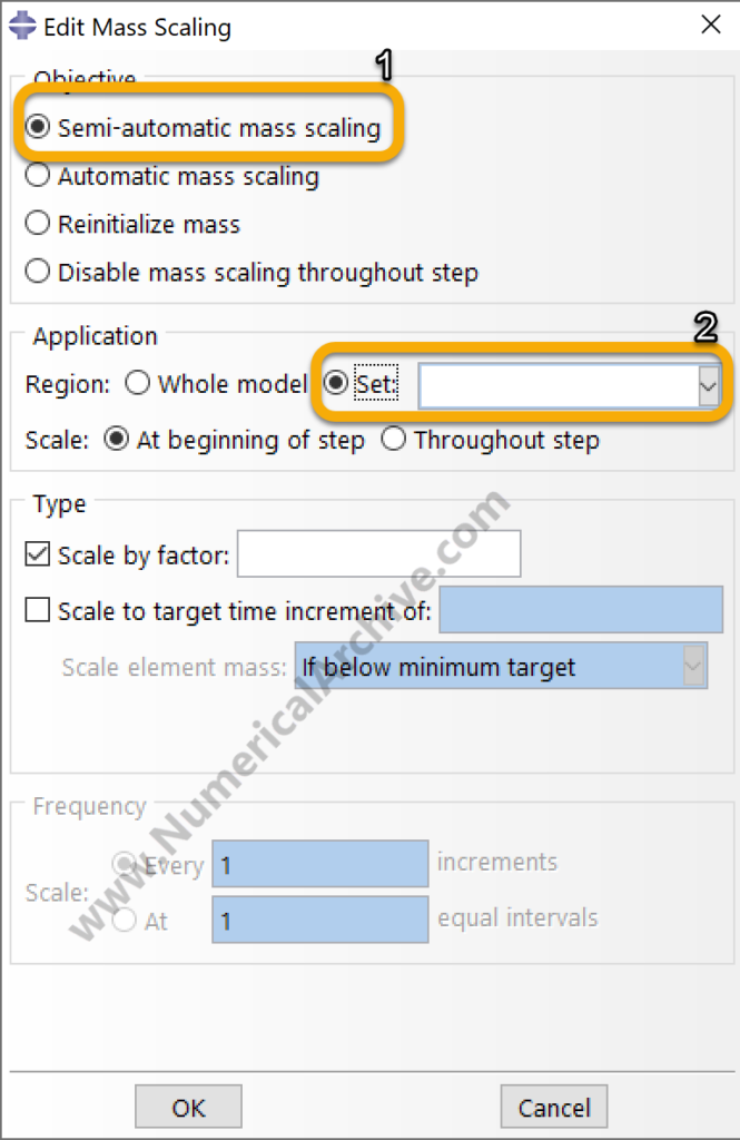
Mass scaling can be applied globally to the full model or locally to an element set. Specifying an element set creates a local mass scaling definition. Omitting the set applies the definition to all applicable elements.

For dynamic simulations and for models with a few isolated controlling elements, local mass scaling is usually easier to justify because the added mass can be confined to the numerical bottleneck. Global mass scaling may be appropriate in some quasi-static simulations, but its effect on inertia and the overall response still needs to be checked.

A global definition and local definitions can be combined. A local mass scaling definition can override the global definition for a specified element set.

The Abaqus/CAE path is:

Step module → Create Step → Dynamic, Explicit → Mass scaling → Create → Semi-automatic mass scaling → Region → Set

How Much Mass Scaling Is Acceptable?

This is the most important practical question—and there is no single mass scaling percentage that is universally acceptable for all Abaqus models.

The correct acceptance criterion depends on the type of analysis and the response being studied. A quasi-static forming simulation, a progressive collapse model, and a high-speed impact analysis do not have the same sensitivity to added mass.

Use the following checks:

• Compare with a baseline: repeat the analysis with less mass scaling and compare the results that support your engineering conclusion.
• Check quasi-static energy behavior: verify that ALLKE remains a small fraction of ALLIE for the quasi-static response.
• Review artificial energy terms: artificial strain energy, damping dissipation, and mass scaling work should remain negligible relative to the physically meaningful energies for the problem.
• Check the added mass distribution: use the element mass scaling factor output EMSF to see where mass has been scaled.
• Review the element stable time increment: use EDT to examine the stable time increment at element level, including the effect of mass scaling.
• Compare response histories: check forces, displacements, accelerations, velocities, stresses, strains, damage variables, and contact quantities relevant to the model.

A mass-scaled result is acceptable when the computational acceleration does not change the engineering conclusion within the accuracy required for the study. The burden of proof is a sensitivity comparison, not a memorized percentage.

Checking ALLKE, ALLIE, and Energy Balance

Energy output is essential when assessing an Abaqus/Explicit analysis.

• ALLKE is the total kinetic energy.
• ALLIE is the total internal energy.
• ETOTAL is the total energy measure used to review overall energy balance.
• ALLMW is the mass scaling work.
• ALLAE is artificial strain energy.
• ALLVD is viscous dissipation associated with damping.

For a quasi-static analysis, kinetic energy should remain small relative to internal energy. For explicit analyses more generally, artificial energy contributions—including mass scaling work—should not dominate the real energy terms. The total energy history should also be physically consistent with the loading and boundary conditions.

Do not inspect only the final value. Plot the energy histories over the full step. Short spikes may correspond to contact initiation, load application, local buckling, fracture, or other physical or numerical events. Interpret the energy curves together with the response history.

Common Mass Scaling Mistakes in Abaqus

1. Applying mass scaling before finding the controlling elements

This can hide a poor-quality element, an unintended tiny edge, or an unnecessarily refined mesh. Diagnose first.

2. Using global mass scaling for a local problem

If ten small elements control a million-element model, adding mass to the entire model is difficult to justify. Create an element set and evaluate local scaling.

3. Using variable mass scaling to hide severe distortion

A shrinking stable time increment can be a symptom of elements becoming highly distorted. Variable mass scaling may keep the job running while the mesh quality continues to deteriorate. Investigate the deformation mechanism and the mesh.

4. Accepting a result only because the job completed

Completion is not validation. Review energy, added mass, critical elements, and the engineering response.

5. Applying aggressive mass scaling in a true dynamic event

Added mass changes inertia. In impact, blast, wave propagation, and other transient problems, compare the mass-scaled solution with a less-scaled reference.

6. Choosing the target time increment by trial and error only

Use the stable time increment report and the distribution of critical elements. A target should address a known numerical bottleneck.

7. Manually changing material density instead of using mass scaling controls

Abaqus mass scaling provides step-based, local, fixed, and variable options and offers dedicated diagnostic outputs. These are more transparent than silently modifying a physical material property.

When You Should Not Use Mass Scaling

Mass scaling is a poor choice when the mass change itself affects the quantity you are trying to predict. Be especially cautious when the analysis depends strongly on:

• natural frequencies or modal content;
• acceleration histories;
• momentum transfer;
• stress-wave propagation;
• high-speed impact response;
• dynamic amplification;
• inertial instability;
• force histories that are highly sensitive to mass.

Mass scaling may still be used selectively in some dynamic models when only a few elements control the time increment, but the effect must be demonstrated to be negligible for the response of interest.

Also avoid mass scaling as the first response to a corrupted mesh, incorrect units, wrong density, unrealistic material stiffness, or severe element distortion. Fix the modeling error before accelerating the analysis.

Mass Scaling vs Mesh Refinement

Mass scaling and mesh modification solve different problems. Mesh refinement is used to improve spatial resolution, represent gradients, capture local behavior, or improve geometric fidelity. Mass scaling is used to improve explicit computational efficiency by modifying mass properties.

If the mesh is unnecessarily fine, coarsening the mesh may increase the stable time increment without changing the physical mass. If a few badly shaped elements control the step, improving the mesh topology may be better than scaling their mass. If local refinement is physically necessary, selective mass scaling may be appropriate after sensitivity checks.

Remember that explicit computational cost grows rapidly with mesh refinement. Refinement increases the number of elements and can simultaneously decrease the stable time increment. This is one reason a few small elements can have a disproportionate effect on runtime.

A Practical Abaqus Mass Scaling Workflow

1. Run the model without aggressive mass scaling. Obtain a baseline or at least a conservative reference case.
2. Inspect the stable time increment. Review the status file and critical-element diagnostics.
3. Locate controlling elements. Identify whether the cause is mesh size, material wave speed, contact, or evolving deformation.
4. Fix modeling problems first. Remove sliver elements, improve mesh transitions, verify units, material data, and contact.
5. Choose fixed or variable scaling. Use fixed scaling for an initial bottleneck and variable scaling when the controlling element size evolves during the step.
6. Prefer local scaling when the problem is local. Create an element set for the controlling region.
7. Increase the target time increment gradually. Avoid jumping directly to an aggressive target.
8. Request diagnostic outputs. Review EMSF, EDT, energy histories, and the critical elements.
9. Compare engineering outputs. Check the quantities that determine your conclusion.
10. Document the sensitivity study. Record the scaling strategy, target increment, affected region, runtime benefit, added mass behavior, and comparison with the reference case.

Abaqus Mass Scaling FAQ

Does mass scaling change the results in Abaqus?

It can. Mass scaling changes mass and therefore can change inertia. The goal is to use a limited and well-targeted amount of scaling so that the response of interest remains insensitive to the numerical modification. A sensitivity comparison is required.

Should I use fixed or variable mass scaling?

Use fixed mass scaling when the controlling small elements exist at the beginning of the step. Consider variable mass scaling when deformation during the step creates or compresses elements that progressively reduce the stable time increment.

What controls the stable time increment in Abaqus/Explicit?

The stability limit is strongly influenced by element characteristic length and dilatational wave speed. Small elements or elements associated with high wave speed can control the initial element-by-element estimate. Contact stiffness and evolving nonlinear behavior can also influence the time increment.

How can I find the elements with the smallest stable time increments?

Review the stable time increment report in the Abaqus .sta file and use the critical-element diagnostic information written to the output database for visualization in Abaqus/CAE.

Is there a maximum acceptable mass scaling percentage?

There is no universal percentage that is valid for every model. Acceptance should be based on energy behavior and sensitivity of the engineering response to a lower-scaling or unscaled reference solution.

What should I check after applying mass scaling?

Review the energy history, especially ALLKE, ALLIE, ETOTAL, and ALLMW. Examine EMSF and EDT, inspect the critical elements, and compare the engineering outputs with a reference case.

Can mass scaling fix distorted elements?

Not by itself. A decreasing stable time increment may occur as elements become compressed or distorted, but mass scaling does not correct bad element geometry. Investigate mesh quality, contact, material behavior, and the deformation mechanism. See our Abaqus common error guide for a broader troubleshooting workflow.

Final Engineering Recommendation

Mass scaling in Abaqus is most effective when it is treated as a controlled numerical strategy rather than a runtime shortcut. Identify the elements controlling the stable time increment, understand why they are controlling the model, apply the minimum necessary scaling to the appropriate region, and verify the response through energy and sensitivity checks.

For quasi-static Abaqus/Explicit analysis, pay particular attention to the relationship between kinetic and internal energy. For dynamic analysis, protect the physical mass and inertia of the model and use local scaling only when its effect on the transient response can be shown to be negligible.

When used with diagnostics, output review, and a reference comparison, mass scaling can reduce explicit analysis time substantially without compromising the engineering conclusions of the model.

Explore the Numerical Archive Abaqus model library for editable numerical models and engineering simulation examples.